Introduction to Hydrodynamic Instability Computational Thermofluid Research Lab
 presented at")
Introduction to Hydrodynamic Instability 黃美嬌 台灣大學機械系 計算熱流研究室 Computational Thermo-fluid Research Lab (CTRL) presented at 東海應數 on Nov. 18, 2004
 Instability")
OUTLINE Overview of hydrodynamic instability Examples: Rayleigh-Benard Instability Taylor (Dean) Instability

Hydrodynamic Instability • Which type, laminar or turbulent, is more likely to occur? laminar when the Reynolds number is very low turbulent at larger Reynolds number • Reynolds number = UL/n = (L 2/n)(L/U)-1 • The equations of hydrodynamics allow some flow patterns. Given a flow pattern , is it stable? If the flow is disturbed, will the disturbance gradually die down, or will the disturbance grow such that the flow departs from its initial state and never recovers?

Free-shear flows: mixing layers, wakes, jets, etc smaller critical Reynolds number less sensitive to the form of the basic flow inviscid instability leads to coherent structures not affected by viscosity if it is small enough Wall-bounded flows: boundary layers, pipe flows, etc basic flows without inflexion point viscosity plays a role sensitive to the form of the basic flow
 ~ incompressible viscous Newtonian flows ~")
Hydrodyanmics ~ n/k = momentum/thermal diffusivities (m 2/sec) ~ incompressible viscous Newtonian flows ~ mass, momentum, energy conservation ~ negligible viscous dissipation heat
 instablility: z x linear stability analysis+normal mode disturbance:")
Kelvin-Helmholtz (inviscid) instablility: z x linear stability analysis+normal mode disturbance:

Kelvin-Helmholtz instablility A long rectangular tube, initially horizontal, is filled with water above colored brine. The fluids are allowed to diffuse for about an hour, and the tube then quickly tilted six degrees, setting the fluids into motion. The brine accelerates uniformly down the slope, while the water above similarly accelerates up the slope. Sinusoidal instability of the interface occurs after a few seconds, and has here grown nonlinearly into regular spiral rolls.
 instablility: ~ instability due to heavy fluid on the upside ~ instability")
Kelvin-Helmholtz (inviscid) instablility: ~ instability due to heavy fluid on the upside ~ instability due to shear ~ instability due to an rapid downward vertical acceleration and heavy fluid rests below ~ instability for all cases
 ~ viscously unstable (Orr-Sommerfeld analysis)")
Wall Shear Flows ~ inviscidly unconditionally stable (Rayleigh analysis) ~ viscously unstable (Orr-Sommerfeld analysis) ~ unstable in labs as Re > 2000

Vortex Shedding

Hope Bifurcation velocity signals vortex shedding behind a vertical plate

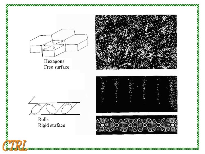
Rayleigh-Benard Instability: Low DT: motionless, pure thermal conduction Higher DT: steady convection roll T Even Higher DT: unsteady, turbulent fluid T+DT q Driving force: buoyancy q Damping force: viscous dissipation

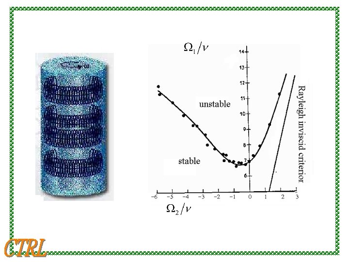
Centrifugal Instability: Low W: laminar, concentric streamlines Higher W: steady convection roll Even Higher W: unsteady, turbulent q Driving force: centrifugal force q Damping force: viscous dissipation W

Görtler Instability d ~ instability due to an imbalance between the centrifugal force and the restoring normal pressure gradient ~ concave walls, e. g. lower side of airfoils; turbine blades
 Görtler number R = radius of curvature")
Görtler Vortex (streamwise vorticity) Görtler number R = radius of curvature

Blasius boundary layer ~ uniform flow over an semi-infinite flat plate ~ Tollmien-Schlichting waves ~ temporary/spatial growth Curves of marginal stability based on the parallel and nonparallel stability theory and experimental data. (temporary instability)

Surface tension instability

Examples: • Rayleigh-Benard instability • Taylor instability

§ Rayleigh-Benard Convection TL H z x TH steady stationary solution under Boussinesq approximation

Linear stability analysis:

characteristic length = H characteristic time = H 2/k characteristic velocity = k/H

Rayleigh number: ~ characteristic frequency of gravity wave Ra = the relative importance of buoyancy effects compared to momentum and thermal diffusive effects.
")
Normal mode approach: Given Pr and Ra, if there exists any mode (kx, ky) such that its (eigenvalue) w has positive imaginary part, then the system is linearly unstable. • free and constant-temperature surfaces: • rigid surfaces:

• free and constant-temperature surfaces:

Ra j=3 j=2 k j=1

H

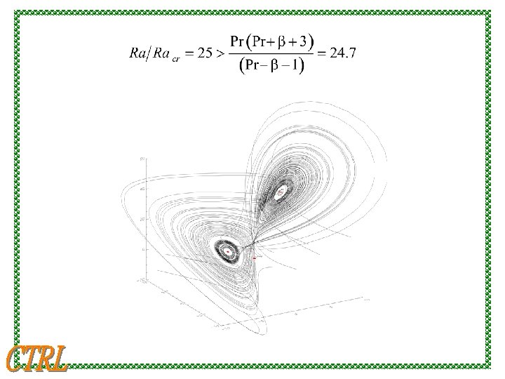
• rigid surfaces: ~ no analytical solution yet ~ numerical solutions available and show As Ra increases, more and more unstable modes are inspired and the flow transition to turbulence via successive bifurcations.

Rayleigh-Benard Instability: Low DT: motionless, pure thermal conduction Higher DT: steady convection roll T Even Higher DT: unsteady, turbulent fluid T+DT q Driving force: buoyancy q Damping force: viscous dissipation

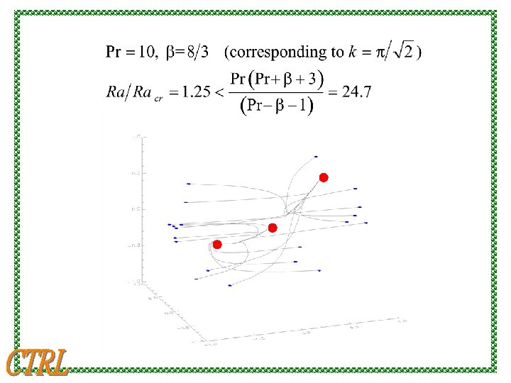
Lorenz: modes with j = 1 X and Y : rising warm fluid and descending cold fluid Z : distortion of the vertical temperature profile from linearity
 = pure (stationary) conduction state ~ the")
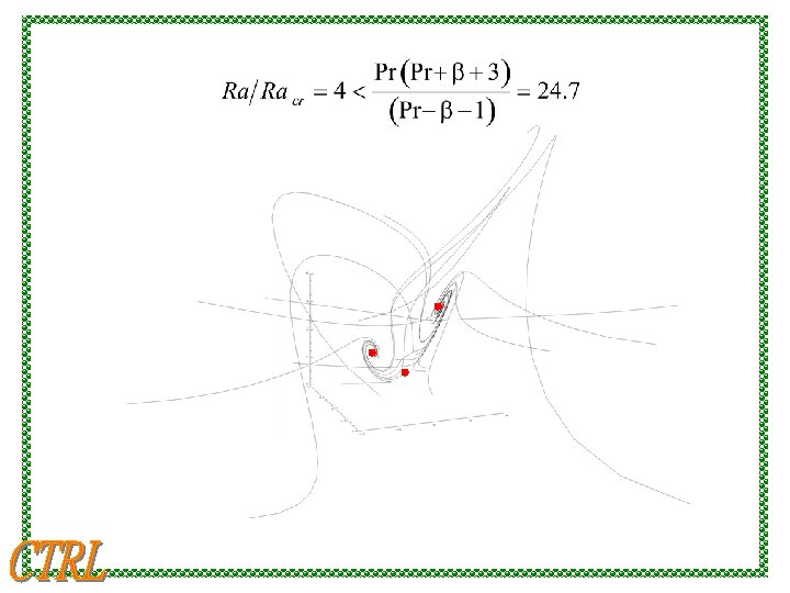
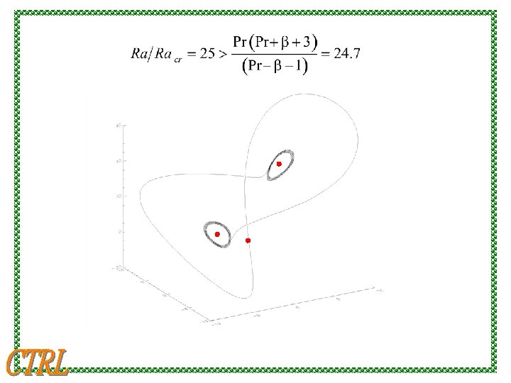
Lorenz equations: Fixed points: (0, 0, 0) = pure (stationary) conduction state ~ the only fixed point if Ra<Racr ~ always exists ~ stable if Ra<Racr ~ unstable if Ra>Racr

Fixed points: ~ exists only if Ra>Racr ~ steady convection roll ~ stable if ~ pitchfork bifurcation at

Taylor Instability: inviscid fluid W

base solution axis-symmetric disturbance ~ Angular momentum per unit mass of a fluid element about the axis (z-axis) remains constant.

motion in the r-z plane: r-direction:pressure force + centrifugal force z-direction:pressure force z r

Centrifugal force = ~ potential-energy-like Consider two fluid particles originally located at r 1 and r 2 respectively and later interchange their locations at later time.

The change in the kinetic energy is azimuthal kinetic energy is released instability possible in the r-z motion

Linear stability analysis: Normal mode approach + axis-symmetric disturbance:

~ classical Sturm-Liouville eigenvalue problem Rayleigh quotient:

Couette Flow W 1 W 2 • Cylinders rotate in the same direction. • Cylinders rotate in different directions.

0. 25 r

r

Viscous damping Taylor number narrow gap approximation:

Hydrodynamic instability ~ free shear ~ wall effect ~ buoyancy-induced ~ stratification effect ~ centrifugal-force induced ~ surface tension ~ others

Figure 1: A stable fluid chain. Figure 2: The instability Figure 3: The same generated by increasing instability visualized flow rate, as seen with the with a strobe lamp. naked eye.

Increasing the flow rate serves to broaden the fishbones.

In the wake of the fluid fish, a regular array of drops obtains, the number and spacing of which is determined by the pinchoff of the fishbones.

polygonal fluid sheet

Thank you for your attention!!

We examine the form of the free surface flows resulting from the collision of equal jets at an oblique angle. Glycerol-water solutions with viscosities of 15 -50 c. S were pumped at flow rates of 10 -40 cc/s through circular outlets with diameter 2 mm. Characteristic flow speeds are 1 -3 m/s. Figures 3 -9 were obtained through strobe illumination at frequencies in the range 2. 5 -10 k. Hz. Figure 1: At low flow rates, the resulting stream takes the form of a steady fluid chain, a succession of mutually orthogonal fluid links, each comprised of a thin oval sheet bound by relatively thick fluid rims. The influence of viscosity serves to decrease the size of successive links, and the chain ultimately coalesces into a cylindrical stream. As the flow rate is increased, waves are excited on the sheet, and the fluid rims become unstable. The rim appears blurred to the naked eye (Figure 2); however, strobe illumination reveals a remarkably regular and striking flow instability ( Figures 3 -6). Droplets form from the sheet rims but remain attached to the fluid sheet by tendrils of fluid that thin and eventually break. The resulting flow takes the form of fluid fishbones, with the fluid sheet being the fish head and the tendrils its bones. Increasing the flow rate serves to broaden the fishbones. Figures 7 -9: In the wake of the fluid fish, a regular array of drops obtains, the number and spacing of which is determined by the pinch-off of the fishbones. Some of these photos have appeared in Hasha & Bush (2002, Phys. Fluids, Gallery of Fluid Motion). A combined theoretical and investigation of fluid chains and fishbones is under review.
- Slides: 55