Introduction to GIS Modeling Week 5 Summarizing Neighborhoods

Introduction to GIS Modeling Week 5 — Summarizing Neighborhoods GEOG 3110 –University of Denver Presented by Joseph K. Berry W. M. Keck Scholar, Department of Geography, University of Denver Calculating slope, aspect and profile maps; Applying spatial differentiation and integration; "Roving window" summary operations; Characterizing edges and complexity

Upcoming Events Exercise #5 — normal report based on Exercise 5 questions; same teams as Exercise 4 report Midterm Study Questions …posted tomorrow by 12: 00 noon (class initiative to “group study” to collectively address the 50+ study questions) Midterm Exam …you will download and take the 2 -hour exam online (honor system) sometime between 10: 00 am Friday February 10 and 5: 00 pm Wednesday February 16 Exercise #6 — you will form your own teams (2 to 4 members) and tackle one of eight projects; posted now but we will discuss all aspects of the project “opportunities” next week …assigned Thursday, February 9 and final report due 5: 00 pm Monday, February 20 No Exercise Week 7 — pause …a moment for a group “dance of joy” Exercises #8 and #9 — to tailor your work to your interests, you can choose to not complete either or both of these standard exercises; in lieu of an exercise, however, you must submit a short paper (4 -8 pages) on a GIS modeling topic of your own choosing Berry

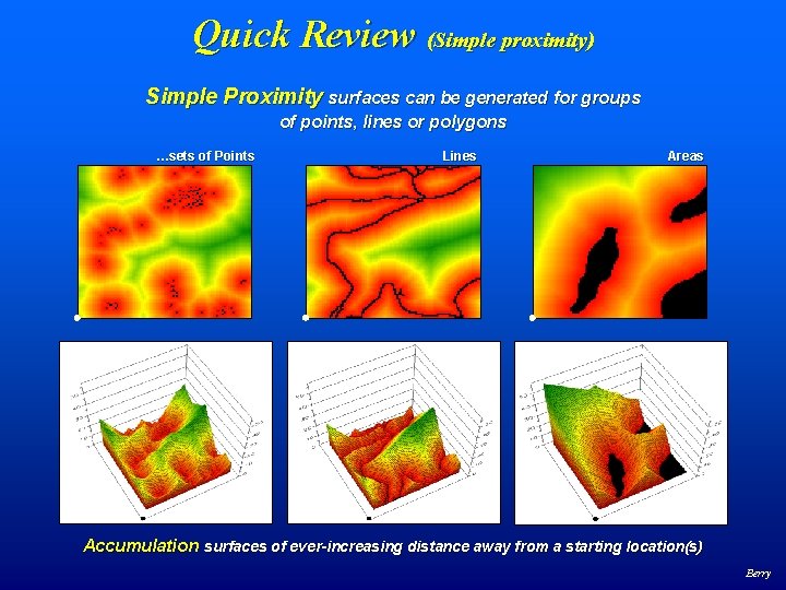
Quick Review (Simple proximity) Simple Proximity surfaces can be generated for groups of points, lines or polygons …sets of Points Lines Areas Accumulation surfaces of ever-increasing distance away from a starting location(s) Berry

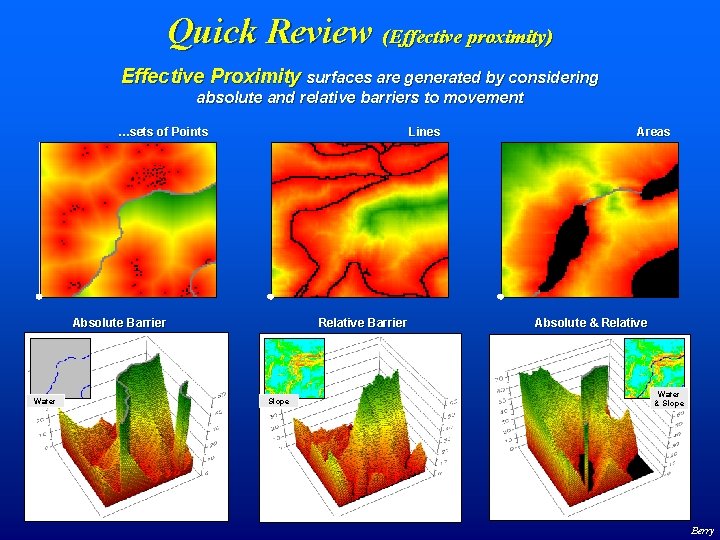
Quick Review (Effective proximity) Effective Proximity surfaces are generated by considering absolute and relative barriers to movement …sets of Points Lines Absolute Barrier Water Relative Barrier Slope Areas Absolute & Relative Water & Slope Berry

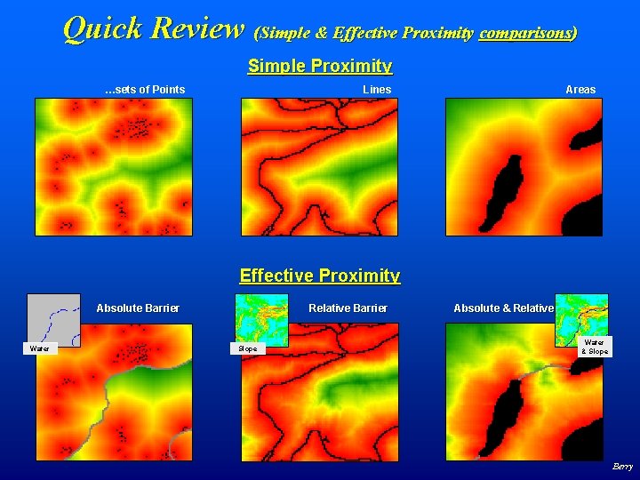
Quick Review (Simple & Effective Proximity comparisons) Simple Proximity …sets of Points Lines Areas Effective Proximity Absolute Barrier Water Relative Barrier Slope Absolute & Relative Water & Slope Berry

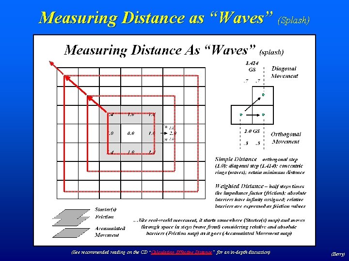
Measuring Distance as “Waves” (Splash) (See recommended reading on the CD “Calculating Effective Distance” for an in-depth discussion) (Berry)

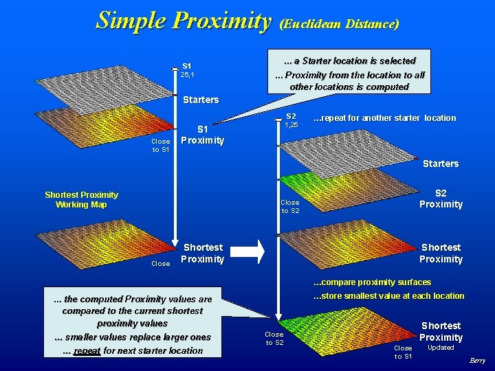
Simple Proximity (Euclidean Distance) S 1 25, 1 … a Starter location is selected … Proximity from the location to all other locations is computed Starters S 2 Close to S 1 1, 25 S 1 Proximity …repeat for another starter location Starters Shortest Proximity Working Map S 2 Proximity Close to S 2 Close Shortest Proximity …compare proximity surfaces …store smallest value at each location … the computed Proximity values are compared to the current shortest proximity values … smaller values replace larger ones … repeat for next starter location Close to S 2 Shortest Proximity Close to S 1 Updated Berry

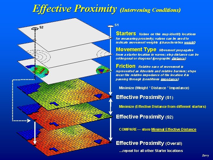
Effective Proximity (Intervening Conditions) S 2 S 1 Starters Values on this map identify locations for measuring proximity; values can be used to indicate movement weights (characteristics weight) Movement Type Movement propagates from a starter location in waves; step distance can be orthogonal or diagonal (geographic distance) Friction Relative ease of movement is represented as Absolute and relative barriers; steps incur the relative impedance of the location it is passing through (conditions impedance) Minimize (Weight * Distance * Impedance) Effective Proximity (S 1) Minimize (Effective Distance from different starters) Effective Proximity (S 2) COMPARE— store Minimal Effective Distance Effective Proximity (Overall) …repeat for all other Starter locations Berry

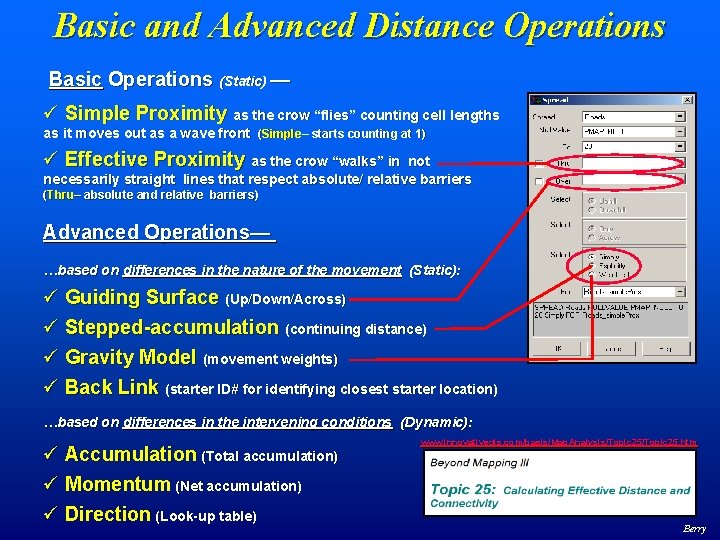
Basic and Advanced Distance Operations Basic Operations (Static) — ü Simple Proximity as the crow “flies” counting cell lengths as it moves out as a wave front (Simple– starts counting at 1) ü Effective Proximity as the crow “walks” in not necessarily straight lines that respect absolute/ relative barriers (Thru– absolute and relative barriers) Advanced Operations— …based on differences in the nature of the movement (Static): ü Guiding Surface (Up/Down/Across) ü Stepped-accumulation (continuing distance) ü Gravity Model (movement weights) ü Back Link (starter ID# for identifying closest starter location) …based on differences in the intervening conditions (Dynamic): ü Accumulation (Total accumulation) ü Momentum (Net accumulation) ü Direction (Look-up table) www. innovativegis. com/basis/Map. Analysis/Topic 25. htm Berry

Basic and Advanced Distance Operations Starters Values on this map identify locations for measuring proximity. Extensions include using the starter value to 1) indicate movement weights, 2) indicate starting distance value and 3) starter location ID# Movement Type Movement propagates from a starter location in waves; step distance can be orthogonal or diagonal (Geographic Distance) Guiding Surface Extension considers 4) whether a step is uphill, downhill or across based on guiding surface configuration Friction Relative ease of movement is represented as Absolute and relative barriers; steps incur the relative impedance of the location it is passing through (Conditions Impedance) Extension uses 5) a look-up table to update the friction surface based on the nature of the movement (direction, accumulation, momentum) Minimize (Distance * Impedance) Effective Proximity Berry

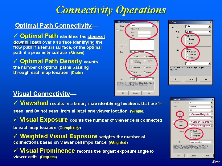
Connectivity Operations Optimal Path Connectivity— ü Optimal Path identifies the steepest downhill path over a surface identifying the flow path if a terrain surface, or the optimal path if a proximity surface (Stream) ü Optimal Path Density counts the number of optimal paths passing through each map location (Drain) Visual Connectivity— ü Viewshed results in a binary map identifying locations that are 1= seen and 0= not seen from at least one viewer location (Simple) ü Visual Exposure counts the number of viewer cells connected to each map location (Completely) <Viewer. Height> <Screen. Heights> <Target. Heights> ü Weighted Visual Exposure weights the number of connections based on viewer cell importance (Weighted) ü Visual Prominence records the largest exposure angle to viewer cells (Degrees) Berry

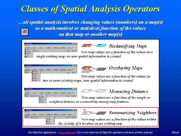
Classes of Spatial Analysis Operators …all spatial analysis involves changing values (numbers) on a map(s) as a mathematical or statistical function of the values on that map or another map(s) (See Map. Calc Applications, “Cross-Reference ” for a cross reference of Map. Calc operations and those of other systems)) “Cross-Reference” (Berry)

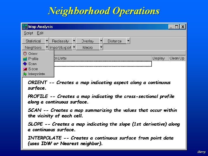
Neighborhood Operations ORIENT -- Creates a map indicating aspect along a continuous surface. PROFILE -- Creates a map indicating the cross-sectional profile along a continuous surface. SCAN -- Creates a map summarizing the values that occur within the vicinity of each cell. SLOPE -- Creates a map indicating the slope (1 st derivative) along a continuous surface. INTERPOLATE -- Creates a continuous surface from point data (uses IDW or Nearest neighbor). (Berry)

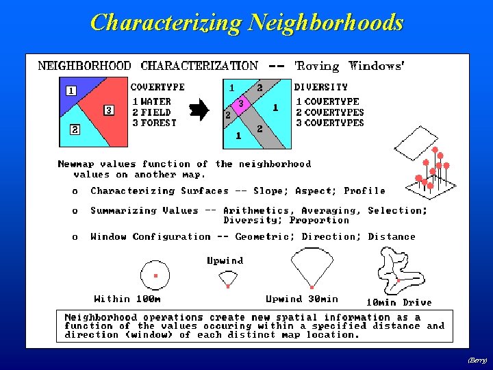
Characterizing Neighborhoods (Berry)

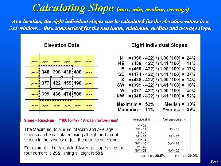
Calculating Slope (max, min, median, average) At a location, the eight individual slopes can be calculated for the elevation values in a 3 x 3 window… then summarized for the maximum, minimum, median and average slope. Slope = Rise/Run (*100 for %) ( Arc. Tan for Degrees) The Maximum, Minimum, Median and Average slopes can be calculated using all eight individual slopes in the window or just the four corner slopes. For example, the calculated Average slope using the four corners is 29%; using all eight is 59%. (Berry)

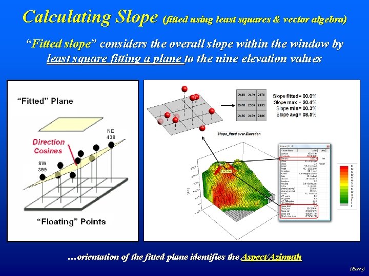
Calculating Slope (fitted using least squares & vector algebra) “Fitted slope” considers the overall slope within the window by least square fitting a plane to the nine elevation values …orientation of the fitted plane identifies the Aspect/Azimuth (Berry)

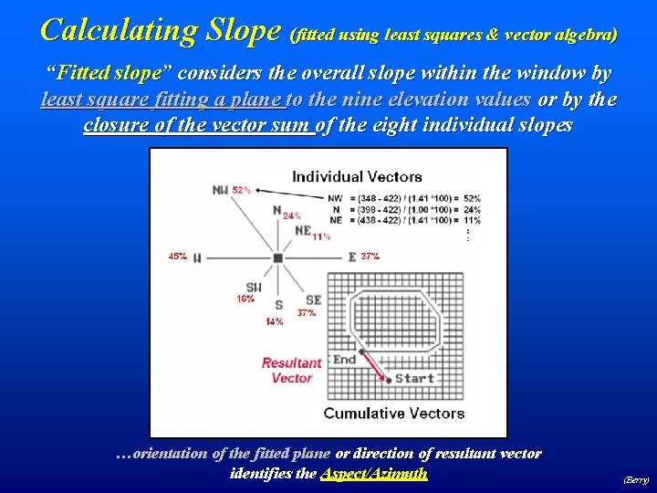
Calculating Slope (fitted using least squares & vector algebra) “Fitted slope” considers the overall slope within the window by least square fitting a plane to the nine elevation values or by the closure of the vector sum of the eight individual slopes …orientation of the fitted plane or direction of resultant vector identifies the Aspect/Azimuth (Berry)

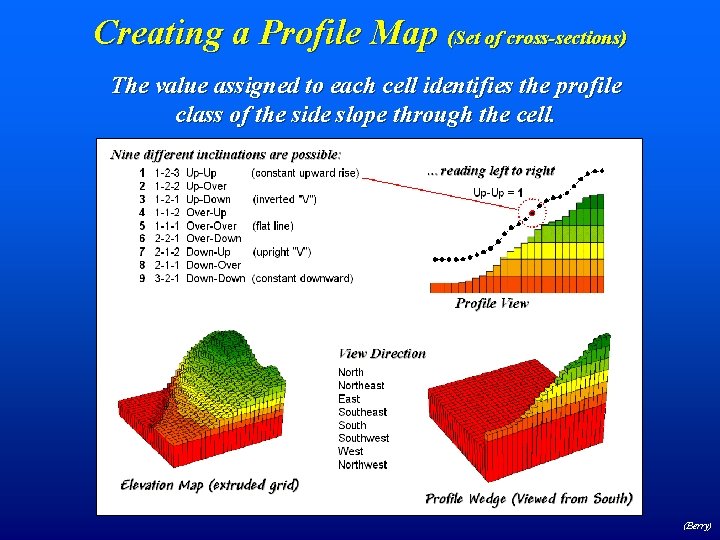
Creating a Profile Map (Set of cross-sections) The value assigned to each cell identifies the profile class of the side slope through the cell. (Berry)

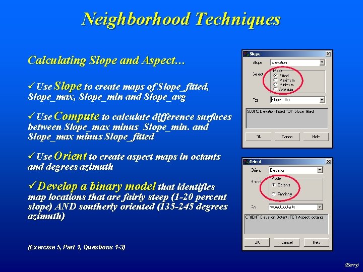
Neighborhood Techniques Calculating Slope and Aspect… üUse Slope to create maps of Slope_fitted, Slope_max, Slope_min and Slope_avg üUse Compute to calculate difference surfaces between Slope_max minus Slope_min. and Slope_max minus Slope_fitted üUse Orient to create aspect maps in octants and degrees azimuth üDevelop a binary model that identifies map locations that are fairly steep (1 -20 percent slope) AND southerly oriented (135 -245 degrees azimuth) (Exercise 5, Part 1, Questions 1 -3) (Berry)

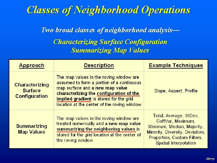
Classes of Neighborhood Operations Two broad classes of neighborhood analysis— Characterizing Surface Configuration Summarizing Map Values (Berry)

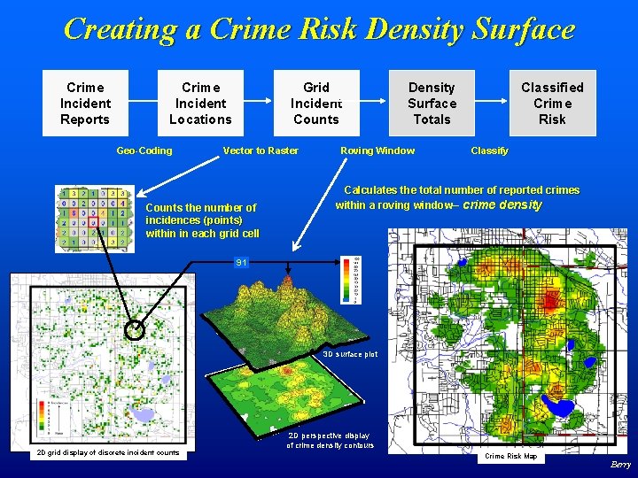
Creating a Crime Risk Density Surface Crime Incident Reports Crime Incident Locations Geo-Coding Grid Incident Counts Vector to Raster Counts the number of incidences (points) within in each grid cell Density Surface Totals Roving Window Classified Crime Risk Classify Calculates the total number of reported crimes within a roving window– crime density 91 3 D surface plot 2 D grid display of discrete incident counts 2 D perspective display of crime density contours Crime Risk Map Berry

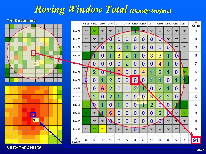
Roving Window Total (Density Surface) # of Customers Customer Density Berry

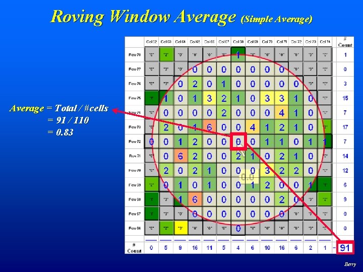
Roving Window Average (Simple Average) Average = Total / #cells = 91 / 110 = 0. 83 Berry

Distance-Weighted Decay Functions Weighted Average of values in the “roving window” Standard mathematical decay functions where weights (Y) decrease with increasing distance (X) Berry

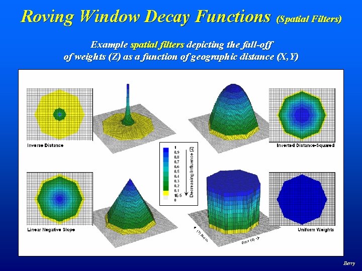
Roving Window Decay Functions (Spatial Filters) Example spatial filters depicting the fall-off of weights (Z) as a function of geographic distance (X, Y) Berry

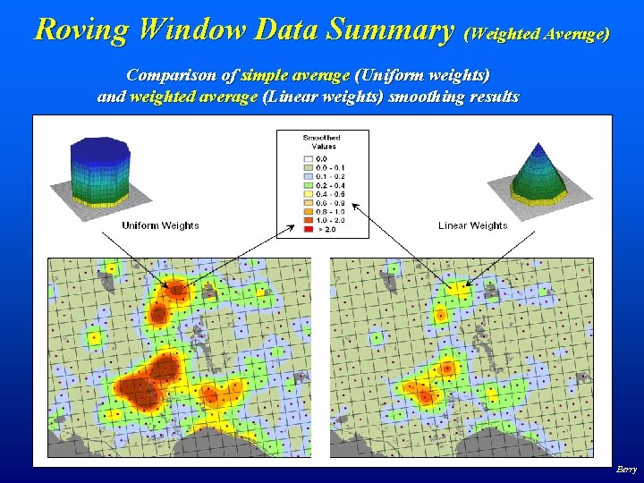
Roving Window Data Summary (Weighted Average) Comparison of simple average (Uniform weights) and weighted average (Linear weights) smoothing results Berry

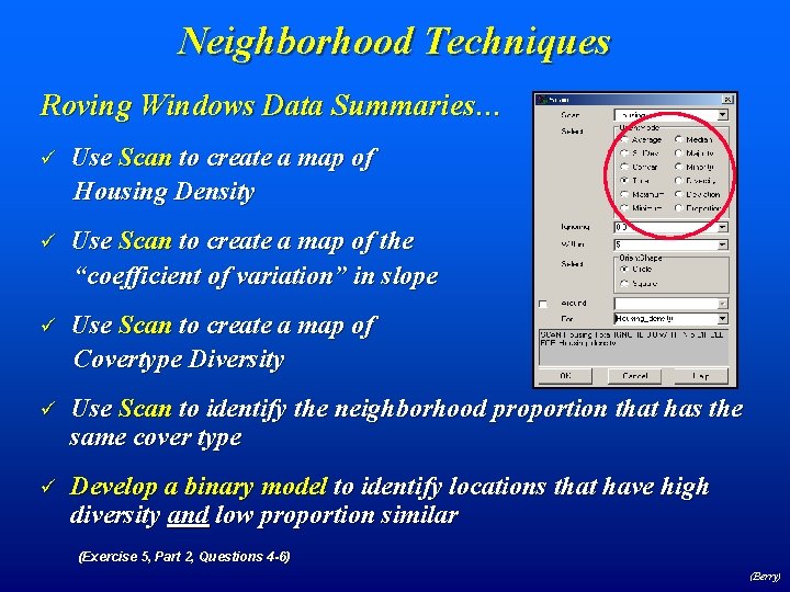
Neighborhood Techniques Roving Windows Data Summaries… ü Use Scan to create a map of Housing Density ü Use Scan to create a map of the “coefficient of variation” in slope ü Use Scan to create a map of Covertype Diversity ü Use Scan to identify the neighborhood proportion that has the same cover type ü Develop a binary model to identify locations that have high diversity and low proportion similar (Exercise 5, Part 2, Questions 4 -6) (Berry)

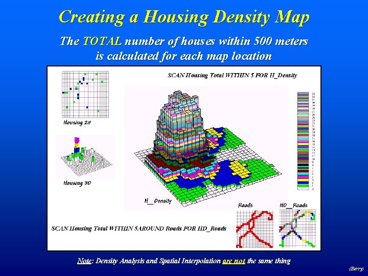
Creating a Housing Density Map The TOTAL number of houses within 500 meters is calculated for each map location Note: Density Analysis and Spatial Interpolation are not the same thing (Berry)

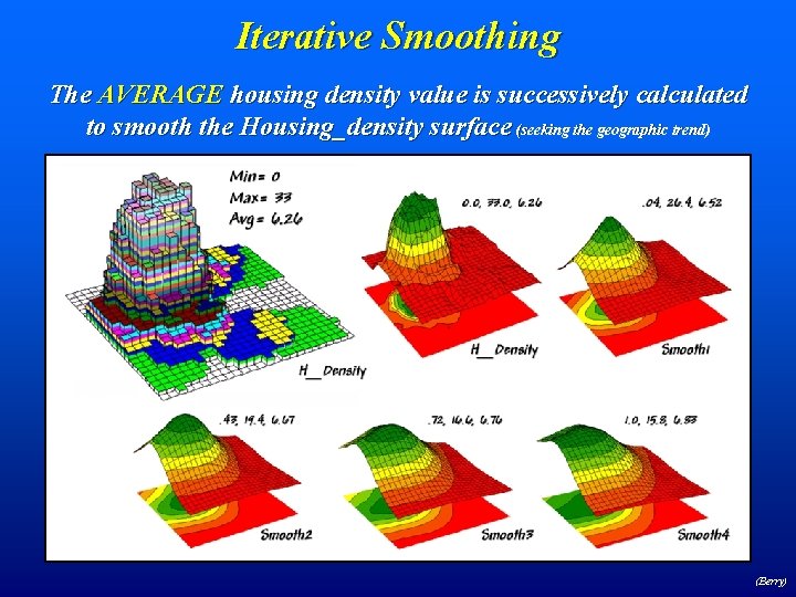
Iterative Smoothing The AVERAGE housing density value is successively calculated to smooth the Housing_density surface (seeking the geographic trend) (Berry)

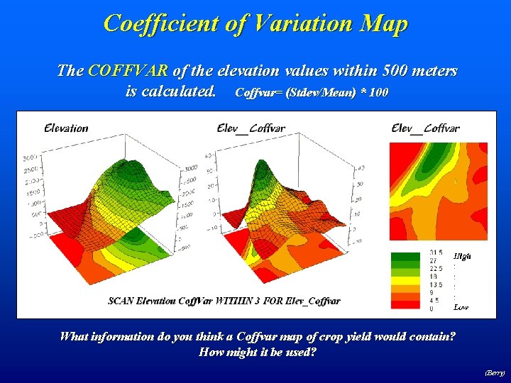
Coefficient of Variation Map The COFFVAR of the elevation values within 500 meters is calculated. Coffvar= (Stdev/Mean) * 100 What information do you think a Coffvar map of crop yield would contain? How might it be used? (Berry)

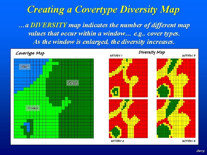
Creating a Covertype Diversity Map …a DIVERSITY map indicates the number of different map values that occur within a window… e. g. , cover types. As the window is enlarged, the diversity increases. (Berry)

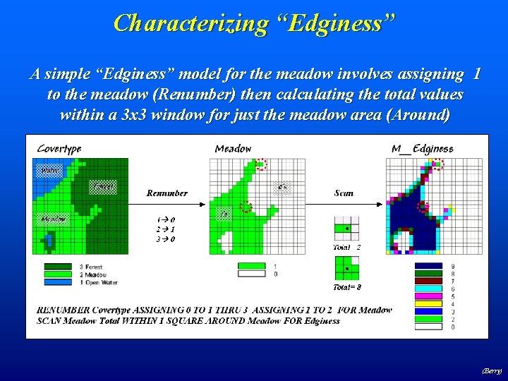
Characterizing “Edginess” A simple “Edginess” model for the meadow involves assigning 1 to the meadow (Renumber) then calculating the total values within a 3 x 3 window for just the meadow area (Around) (Berry)