Introduction to GIS Modeling Week 4 Measuring Distance

Introduction to GIS Modeling Week 4 — Measuring Distance and Connectivity GEOG 3110 –University of Denver Presented by Joseph K. Berry W. M. Keck Scholar, Department of Geography, University of Denver Simple vs. weighted distance; Proximity and movement; Accumulation surfaces; Identifying optimal path(s); Narrowness; Viewsheds and visual exposure surfaces

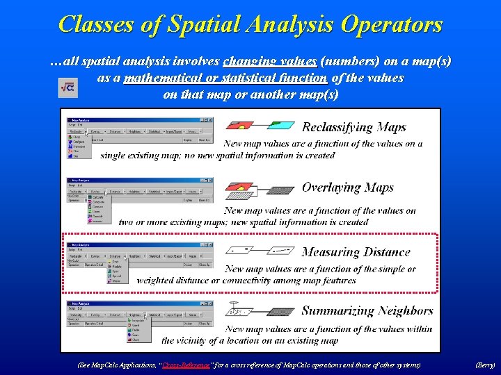
Classes of Spatial Analysis Operators …all spatial analysis involves changing values (numbers) on a map(s) as a mathematical or statistical function of the values on that map or another map(s) (See Map. Calc Applications, “Cross-Reference ” for a cross reference of Map. Calc operations and those of other systems) “Cross-Reference” (Berry)

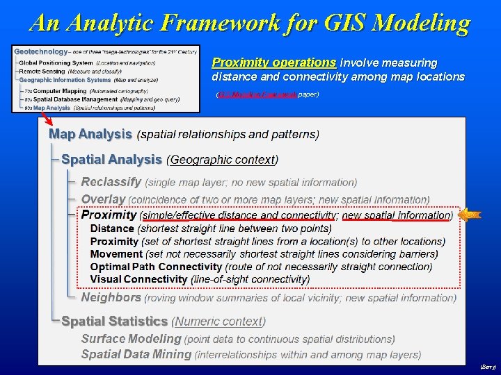
An Analytic Framework for GIS Modeling Proximity operations involve measuring distance and connectivity among map locations (GIS Modeling Framework paper) (Berry)

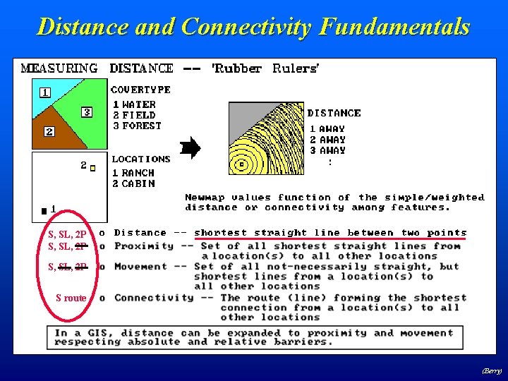
Distance and Connectivity Fundamentals S, SL, 2 P S route (Berry)

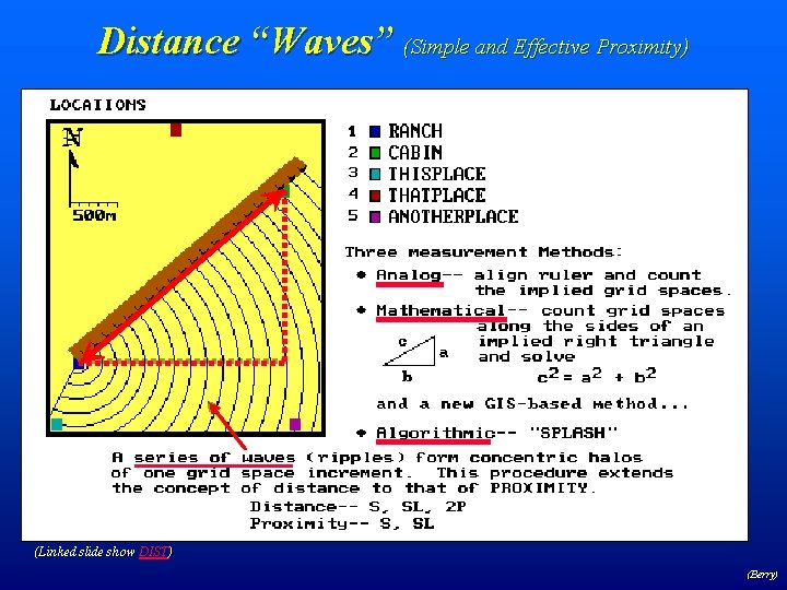
Distance “Waves” (Simple and Effective Proximity) (Linked slide show DIST) (Berry)

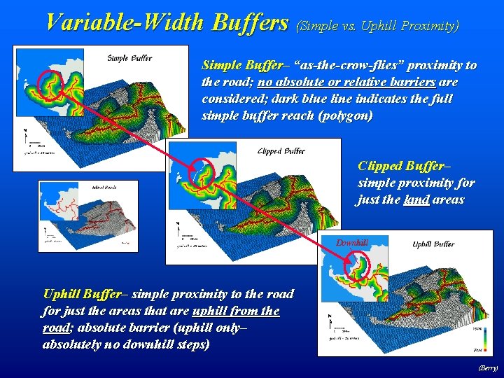
Variable-Width Buffers (Simple vs. Uphill Proximity) Simple Buffer– “as-the-crow-flies” proximity to the road; no absolute or relative barriers are considered; dark blue line indicates the full simple buffer reach (polygon) Clipped Buffer– simple proximity for just the land areas Downhill Uphill Buffer– simple proximity to the road for just the areas that are uphill from the road; absolute barrier (uphill only– absolutely no downhill steps) (Berry)

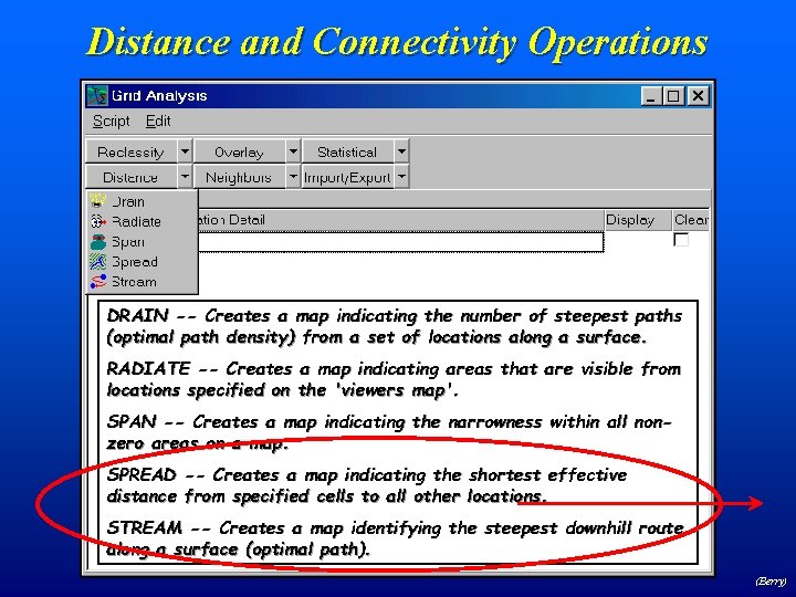
Distance and Connectivity Operations DRAIN -- Creates a map indicating the number of steepest paths (optimal path density) from a set of locations along a surface. RADIATE -- Creates a map indicating areas that are visible from locations specified on the 'viewers map'. SPAN -- Creates a map indicating the narrowness within all nonzero areas on a map. SPREAD -- Creates a map indicating the shortest effective distance from specified cells to all other locations. STREAM -- Creates a map identifying the steepest downhill route along a surface (optimal path). (Berry)

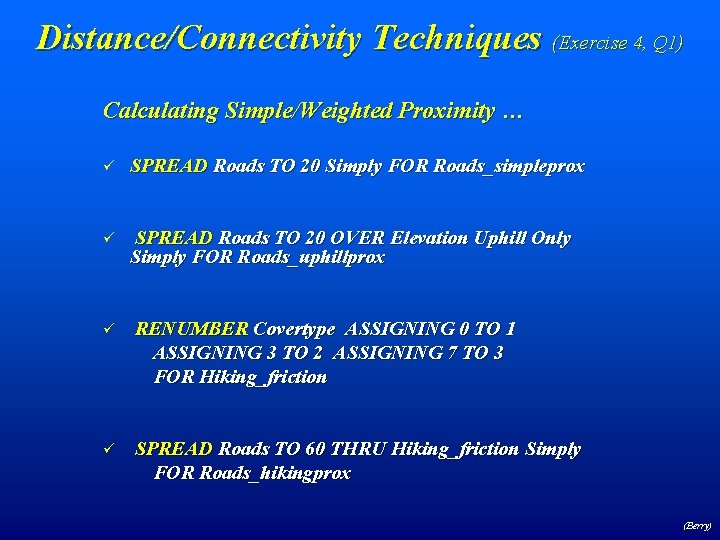
Distance/Connectivity Techniques (Exercise 4, Q 1) Calculating Simple/Weighted Proximity … ü SPREAD Roads TO 20 Simply FOR Roads_simpleprox ü SPREAD Roads TO 20 OVER Elevation Uphill Only Simply FOR Roads_uphillprox ü RENUMBER Covertype ASSIGNING 0 TO 1 ASSIGNING 3 TO 2 ASSIGNING 7 TO 3 FOR Hiking_friction ü SPREAD Roads TO 60 THRU Hiking_friction Simply FOR Roads_hikingprox (Berry)

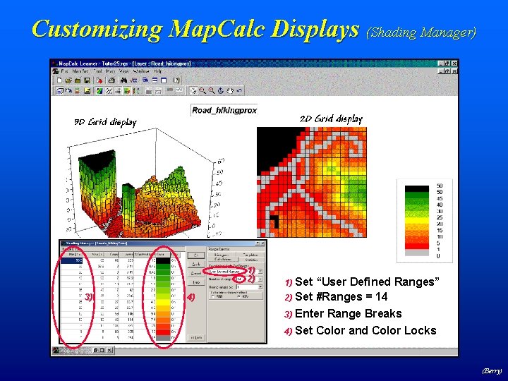
Customizing Map. Calc Displays (Shading Manager) 1) 2) 3) 4) Set “User Defined Ranges” 2) Set #Ranges = 14 1) Enter Range Breaks 4) Set Color and Color Locks 3) (Berry)

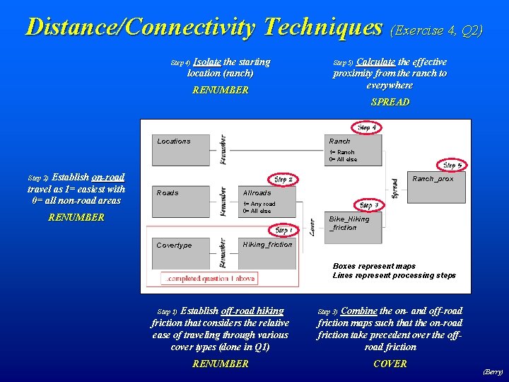
Distance/Connectivity Techniques (Exercise 4, Q 2) Isolate the starting location (ranch) Step 4) RENUMBER Calculate the effective proximity from the ranch to everywhere Step 5) SPREAD Ranch Locations 1= Ranch 0= All else Establish on-road travel as 1= easiest with 0= all non-road areas Step 2) Ranch_prox Roads Allroads 1= Any road 0= All else RENUMBER Bike_Hiking _friction Covertype Hiking_friction Boxes represent maps Lines represent processing steps Establish off-road hiking friction that considers the relative ease of traveling through various cover types (done in Q 1) Step 1) RENUMBER Combine the on- and off-road friction maps such that the on-road friction take precedent over the offroad friction Step 3) COVER (Berry)

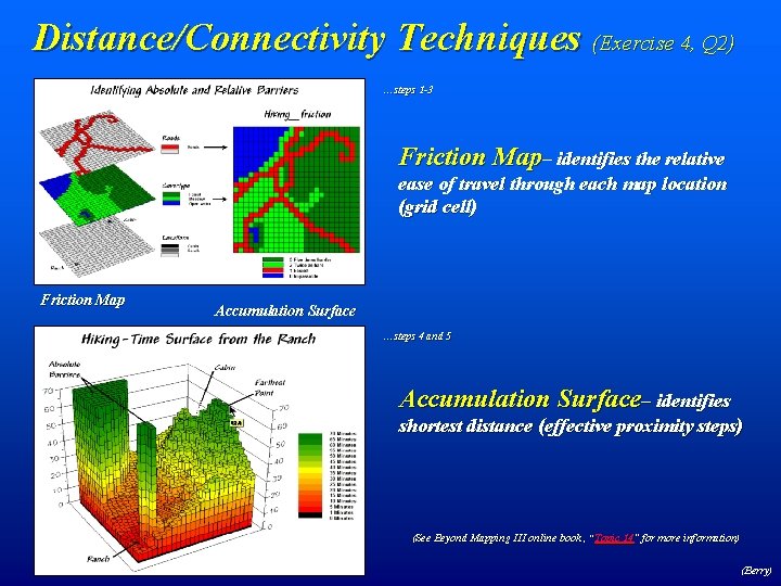
Distance/Connectivity Techniques (Exercise 4, Q 2) …steps 1 -3 Friction Map– identifies the relative ease of travel through each map location (grid cell) Friction Map Accumulation Surface …steps 4 and 5 Accumulation Surface– identifies 83. 0 shortest distance (effective proximity steps) (See Beyond Mapping III online book , “Topic 14” for more information) (Berry)

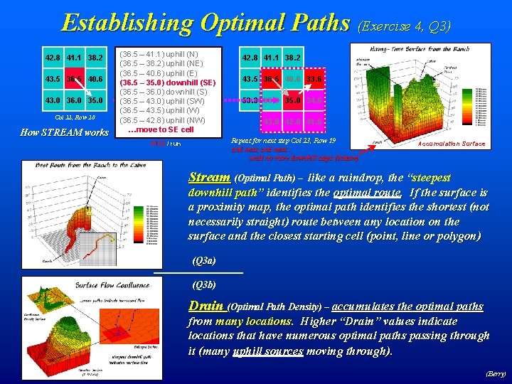
Establishing Optimal Paths (Exercise 4, Q 3) 42. 8 41. 1 38. 2 43. 5 36. 5 40. 6 43. 0 36. 0 35. 0 Col 22, Row 20 How STREAM works (36. 5 – 41. 1) uphill (N) (36. 5 – 38. 2) uphill (NE) (36. 5 – 40. 6) uphill (E) (36. 5 – 35. 0) downhill (SE) (36. 5 – 36. 0) downhill (S) (36. 5 – 43. 0) uphill (SW) (36. 5 – 43. 5) uphill (W) (36. 5 – 42. 8) uphill (NW) …move to SE cell 42. 8 41. 1 38. 2 43. 5 36. 5 40. 6 33. 6 50. 0 36. 0 35. 0 34. 6 43. 0 42. 0 41. 6 Repeat for next step Col 23, Row 19 and next, and next… until no more downhill steps (bottom) RISE / run Accumulation Surface Stream (Optimal Path) – like a raindrop, the “steepest downhill path” identifies the optimal route. If the surface is a proximity map, the optimal path identifies the shortest (not necessarily straight) route between any location on the surface and the closest starting cell (point, line or polygon) (Q 3 a) (Q 3 b) Drain (Optimal Path Density) – accumulates the optimal paths from many locations. Higher “Drain” values indicate locations that have numerous optimal paths passing through it (many uphill sources moving through). (Berry)

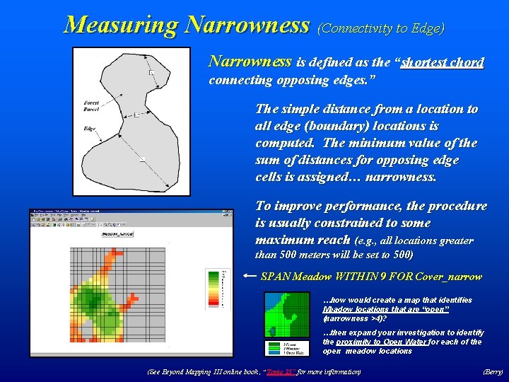
Measuring Narrowness (Connectivity to Edge) Narrowness is defined as the “shortest chord connecting opposing edges. ” The simple distance from a location to all edge (boundary) locations is computed. The minimum value of the sum of distances for opposing edge cells is assigned… narrowness. To improve performance, the procedure is usually constrained to some maximum reach (e. g. , all locations greater than 500 meters will be set to 500) SPAN Meadow WITHIN 9 FOR Cover_narrow …how would create a map that identifies Meadow locations that are “open” (narrowness >4)? …then expand your investigation to identify the proximity to Open Water for each of the open meadow locations (See Beyond Mapping III online book , “Topic 25” for more information) (Berry)

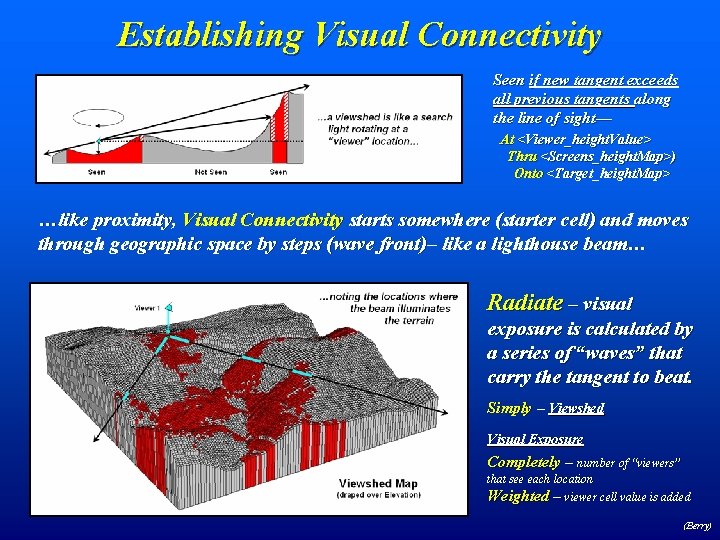
Establishing Visual Connectivity Seen if new tangent exceeds all previous tangents along the line of sight— At <Viewer_height. Value> Thru <Screens_height. Map>) Onto <Target_height. Map> …like proximity, Visual Connectivity starts somewhere (starter cell) and moves through geographic space by steps (wave front)– like a lighthouse beam… Radiate – visual exposure is calculated by a series of “waves” that carry the tangent to beat. Simply – Viewshed Visual Exposure Completely – number of “viewers” that see each location Weighted – viewer cell value is added (Berry)

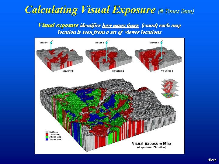
Calculating Visual Exposure (# Times Seen) Visual exposure identifies how many times (count) each map location is seen from a set of viewer locations (Berry)

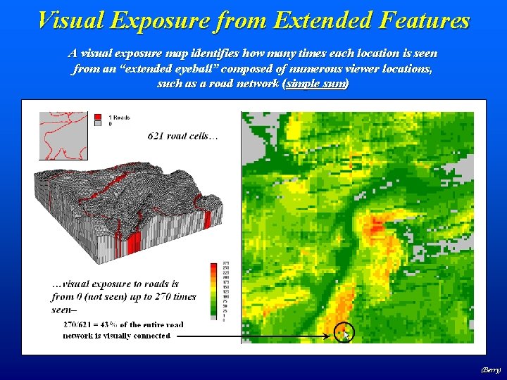
Visual Exposure from Extended Features A visual exposure map identifies how many times each location is seen from an “extended eyeball” composed of numerous viewer locations, such as a road network (simple sum) (Berry)

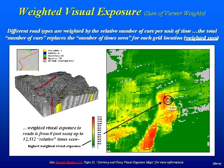
Weighted Visual Exposure (Sum of Viewer Weights) Different road types are weighted by the relative number of cars per unit of time …the total “number of cars” replaces the “number of times seen” for each grid location (weighted sum) (See Beyond Mapping III, Topic 15, “Deriving and Using Visual Exposure Maps” for more information) (Berry)

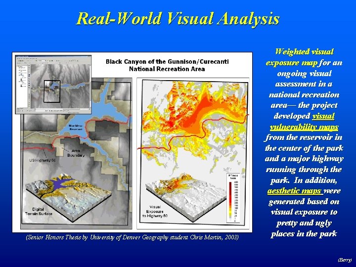
Real-World Visual Analysis (Senior Honors Thesis by University of Denver Geography student Chris Martin, 2003) Weighted visual exposure map for an ongoing visual assessment in a national recreation area— the project developed visual vulnerability maps from the reservoir in the center of the park and a major highway running through the park. In addition, aesthetic maps were generated based on visual exposure to pretty and ugly places in the park (Berry)

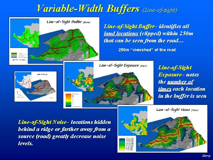
Variable-Width Buffers (Line-of-sight) Line-of-Sight Buffer– identifies all land locations (clipped) within 250 m that can be seen from the road… 250 m “viewshed” of the road Line-of-Sight Exposure– notes the number of times each location in the buffer is seen Line-of-Sight Noise– locations hidden behind a ridge or farther away from a source (road) greatly decrease noise levels. (Berry)

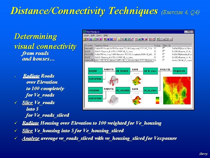
Distance/Connectivity Techniques (Exercise 4, Q 4) Determining visual connectivity from roads and houses… ü ü ü Radiate Roads over Elevation to 100 completely for Ve_roads Slice Ve_roads into 5 for Ve_roads_sliced Radiate Housing over Elevation to 100 weighted for Ve_housing Slice Ve_housing into 5 for Ve_housing_sliced Analyze average ve_roads_sliced with ve_housing_sliced for Vexposure (Berry)

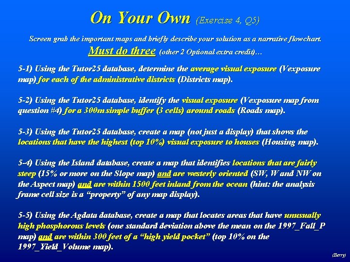
On Your Own (Exercise 4, Q 5) Screen grab the important maps and briefly describe your solution as a narrative flowchart. Must do three (other 2 Optional extra credit)… 5 -1) Using the Tutor 25 database, determine the average visual exposure (Vexposure map) for each of the administrative districts (Districts map). 5 -2) Using the Tutor 25 database, identify the visual exposure (Vexposure map from question #4) for a 300 m simple buffer (3 cells) around roads (Roads map). 5 -3) Using the Tutor 25 database, create a map (not just a display) that shows the locations that have the highest (top 10%) visual exposure to houses (Housing map). 5 -4) Using the Island database, create a map that identifies locations that are fairly steep (15% or more on the Slope map) and are westerly oriented (SW, W and NW on the Aspect map) and are within 1500 feet inland from the ocean (hint: the analysis frame cell size is a “property” of any map display). 5 -5) Using the Agdatabase, create a map that locates areas that have unusually high phosphorous levels (one standard deviation above the mean on the 1997_Fall_P map) and are within 300 feet of a “high yield pocket” (top 10% on the 1997_Yield_Volume map). (Berry)

Optional Questions Extended “Problems with No Guidance” Weighted Visual Exposure Density Surface “Draining Forests” for What? (Berry)

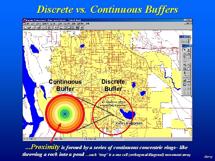
Discrete vs. Continuous Buffers Continuous Buffer Discrete Buffer …all locations within a specified distance …Proximity is formed by a series of continuous concentric rings– like throwing a rock into a pond …each “step” is a one cell (orthogonal/diagonal) movement away (Berry)

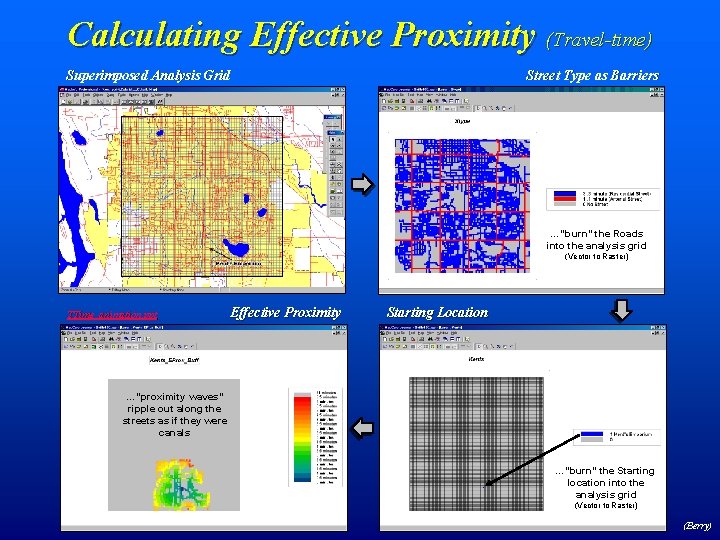
Calculating Effective Proximity (Travel-time) Superimposed Analysis Grid Street Type as Barriers Streets are calibrated… …for ease of …“burn” the Roads travel… into the analysis grid (Vector to Raster) 100 c x 100 r = 10, 000 cells TTime_animation. ppt Effective Proximity …”proximity waves” ripple out along the streets as if they were canals Starting Location …splash… …minutes away …”burn” the Starting location into the analysis grid (Vector to Raster) (Berry)

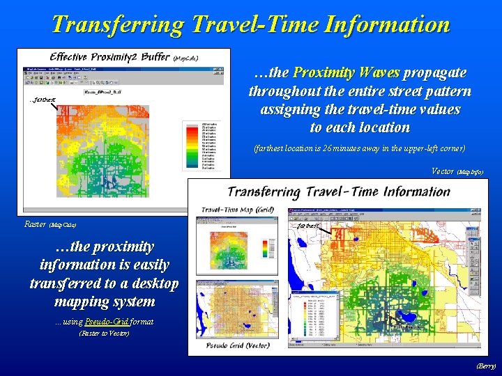
Transferring Travel-Time Information …the Proximity Waves propagate throughout the entire street pattern assigning the travel-time values to each location . . . farthest (farthest location is 26 minutes away in the upper-left corner) Vector (Map. Info) Raster (Map. Calc) . . . farthest …the proximity information is easily transferred to a desktop mapping system …using Pseudo-Grid format (Raster to Vector) (Berry)

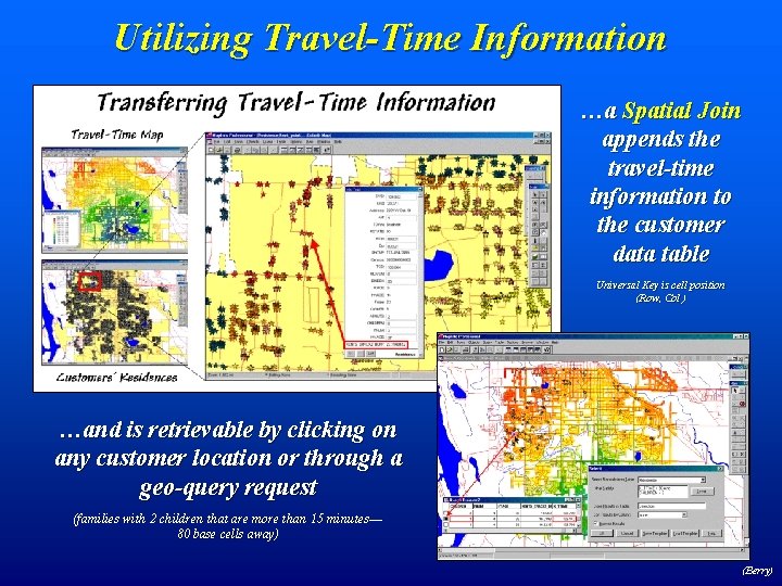
Utilizing Travel-Time Information …a Spatial Join appends the travel-time information to the customer data table Universal Key is cell position (Row, Col ) …and is retrievable by clicking on any customer location or through a geo-query request (families with 2 children that are more than 15 minutes— 80 base cells away) (Berry)

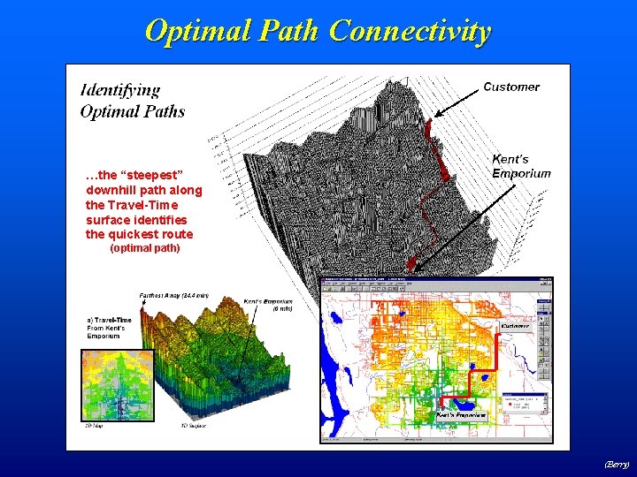
Optimal Path Connectivity …the “steepest” downhill path along the Travel-Time surface identifies the quickest route (optimal path) (Berry)

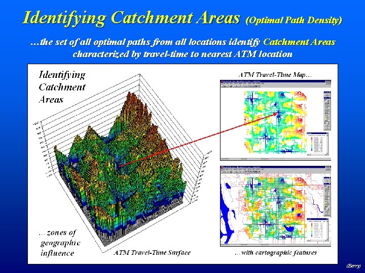
Identifying Catchment Areas (Optimal Path Density) …the set of all optimal paths from all locations identify Catchment Areas characterized by travel-time to nearest ATM location (Berry)

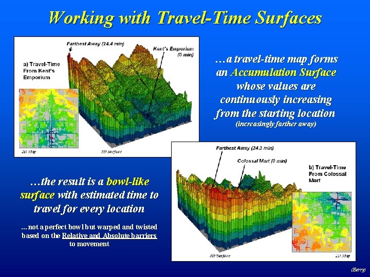
Working with Travel-Time Surfaces …a travel-time map forms an Accumulation Surface whose values are continuously increasing from the starting location (increasingly farther away) …the result is a bowl-like surface with estimated time to travel for every location …not a perfect bowl but warped and twisted based on the Relative and Absolute barriers to movement (Berry)

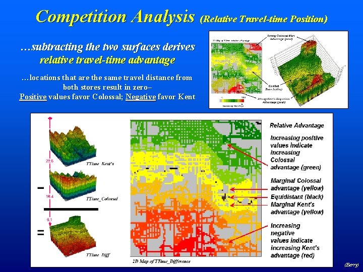
Competition Analysis (Relative Travel-time Position) …subtracting the two surfaces derives relative travel-time advantage …locations that are the same travel distance from both stores result in zero– Positive values favor Colossal; Negative favor Kent (Berry)