Introduction to Gene Mapping Techniques Lecture 2 Background

Introduction to Gene Mapping Techniques Lecture 2 Background Readings: Chapter 5 & 6 (190 -193) of An introduction to Genetics, Griffiths et al. 2000, Seventh Edition. This class has been edited from several sources. Primarily from Terry Speed’s homepage at Stanford and the Technion course “Introduction to Genetics”. Changes made by Dan Geiger. .
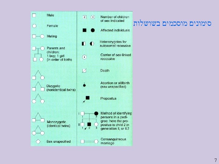
 Male or female Recombination Haplotype : תאי מין או")
Recombination Phenomenon (Happens during Meiosis) Male or female Recombination Haplotype : תאי מין או זרע , ביצית 2

Homolog chromosomes showing Chaismata כרומוזומים הומולוגיים המראים כיאסמתה Sister chromatids . הכיאסמה היא הביטוי הציטולוגי לשחלוף Chaisma(ta) is the cellular expression of recombination. 3
: 2, 839 flies Eye color A: red Wing length")
Morgan’s fruit fly data (1909): 2, 839 flies Eye color A: red Wing length B: normal a: purple b: vestigial AABB aabb x Aa. Bb Expected Observed Aa. Bb 710 1, 339 x Aabb 710 151 aabb aa. Bb 710 154 aabb 710 1, 195 The pair AB stick together more than expected from Mendel’s law: RF =(151+154)/2839=0. 107 4

The Chi-Square test Bb Aa aa 1339 154 bb 151 1490 1195 1349 1493 1346 2839 Expected means under assumption of independence of the loci A and B. Using 2 tables, with one degree of freedom, this number is converted to a probability. If the probability is less than 0. 05, the null hypothesis of independence is rejected. Use with care; the conversion to probability encodes technical assumptions. This translates to a tiny probability not appearing in the tables; so independence is strongly rejected. 5

Example: ABO, AK 1 on Chromosome 9 A A 1/A 1 2 1 O O O A 2 A 2/A 2 Phase inferred A O A 1 A 2 Recombinant A A 1/A 2 4 3 O O A 1 A 2 O A A 2/A 2 A |O A 2 | A 2 5 A 1/A 2 Recombination fraction is 12/100 in males and 20/100 in females. One centi-morgan means one recombination every 100 meiosis. One centi-morgan corresponds to approx 1 M nucleotides (with large variance) depending on location and sex. 6
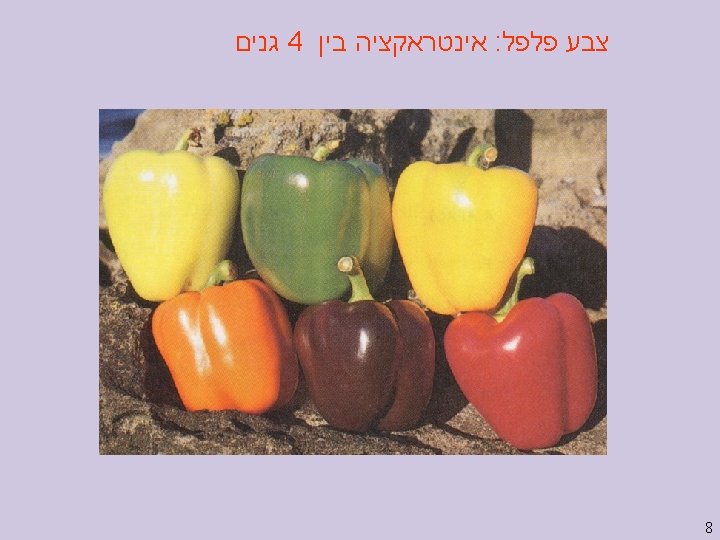

גנים 4 אינטראקציה בין : צבע פלפל Y : removal of green chlorophyll from fruit y : green chlorophyll in fruit R : Red carotenoid pigment r : yellow carotenoid pigment C 1; C 2 : Two genes with the same function, determine amount of carotenoids. c 1; c 2 : Recessive mutations, lower the amount of carotenoids. Genotype Phenotype r/r C 1/C 1 C 2/C 2 y/y green R/R C 1/C 1 C 2/C 2 Y/Y red R/R C 1/C 1 C 2/C 2 y/y brown r/r C 1/C 1 C 2/C 2 Y/Y yellow R/R C 1/C 1 c 2/c 2 Y/Y orange r/r c 1/c 1 c 2/c 2 Y/Y white 9

Purpose of human linkage analysis To obtain a crude chromosomal location of the gene or genes associated with a phenotype of interest, e. g. a genetic disease or an important quantitative trait. Examples: Cystic fibrosis (found), Diabetes, Alzheimer, and Blood pressure. 11
 l l l Linkage")
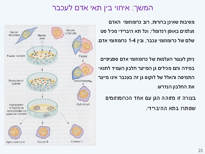
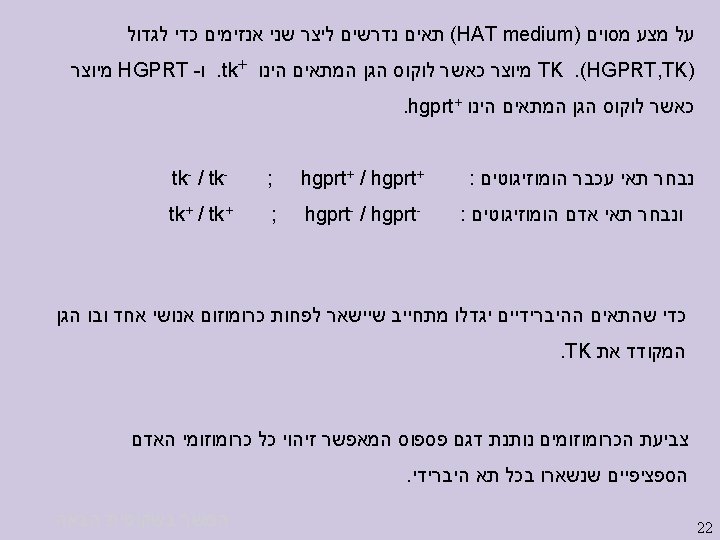
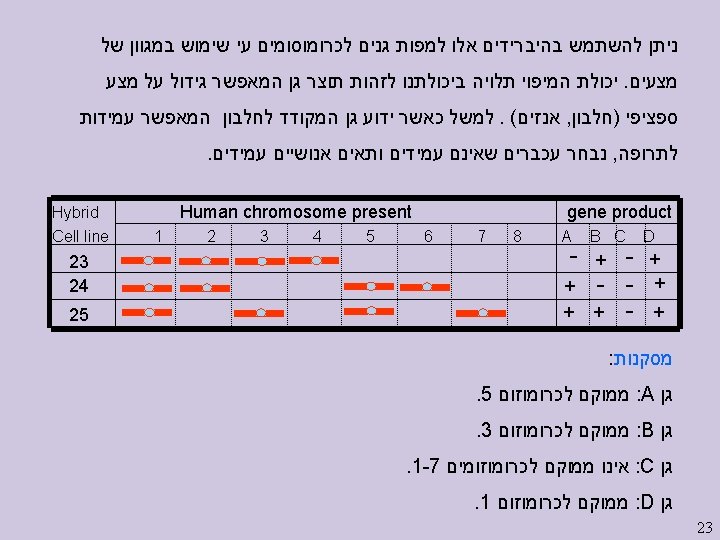
Linkage Strategies I Traditional (from the 1980 s or earlier) l l l Linkage analysis on pedigrees Association studies: candidate genes Allele-sharing methods: Affected siblings Animal models: identifying candidate genes Cell – hybrids Newer (from the 1990 s) l l Focus on special populations (Finland, Hutterites) Haplotype-sharing (many variants) 12

Linkage analysis 13

Fictitious Example for Finding Disease Genes H A 1/A 1 2 1 D D D A 2 A 2/A 2 Phase inferred H D A 1 A 2 Recombinant H A 1/A 2 4 3 D D A 1 A 2 D H A 2/A 2 H |D A 2 | A 2 5 A 1/A 2 We use a marker with codominant alleles A 1/A 2. We speculate a locus with alleles H (Healthy) / D (affected) If the expected number of recombinants is low (close to zero), then the speculated locus and the marker are tentatively physically closed. 14

Association Studies 15
 X x H A f. XH f.")
Healthy/Affected versus a bi-allelic Marker (X, x) X x H A f. XH f. XA f. X 78 72 150 fx. H fx. A fx 44 41 85 f. H f. A f 122 113 235 So healthy status seems independent of marker X. 16

The Chi-Square test H X f. XH f. XA 78 x A 72 fx. H fx. A f. X 150 fx 44 41 85 f. H f. A f 122 113 235 Expected means under assumption of independence of H/A versus X/x. Using 2 tables, the assertion of independence not is rejected in this example; the probability of 2 is much higher than 0. 05. 17

Allele-sharing methods 18

Animal/Plant Breeding Methods Inappropriate for humans. Not practical for large mammals. Not covered in this course, which focuses on computation related to human genetics. 19
 l l Single-nucleotide polymorphism (SNPs) Functional analyses:")
Linkage Strategies II On the horizon (here) l l Single-nucleotide polymorphism (SNPs) Functional analyses: finding candidate genes Needed (starting to happen) l l New multilocus analysis techniques, especially Ways of dealing with large pedigrees Better phenotypes: ones closer to gene products Large collaborations 24

Horses for courses u Each of these strategies has its domain of applicability u Each of them has a different theoretical basis and method of analysis u Which is appropriate for mapping genes for a disease of interest depends on a number of matters, most importantly the disease, and the population from which the sample comes. 25
, prevalence, features such as age at onset Genetics: nature")
The disease matters Definition (phenotype), prevalence, features such as age at onset Genetics: nature of genes (Penetrance), number of genes, nature of their contributions (additive, interacting), size of effect Other relevant variables: Sex, obesity, etc. Genotype-by-environment interactions: Exposure to sun. 26

Example: Age at onset 27

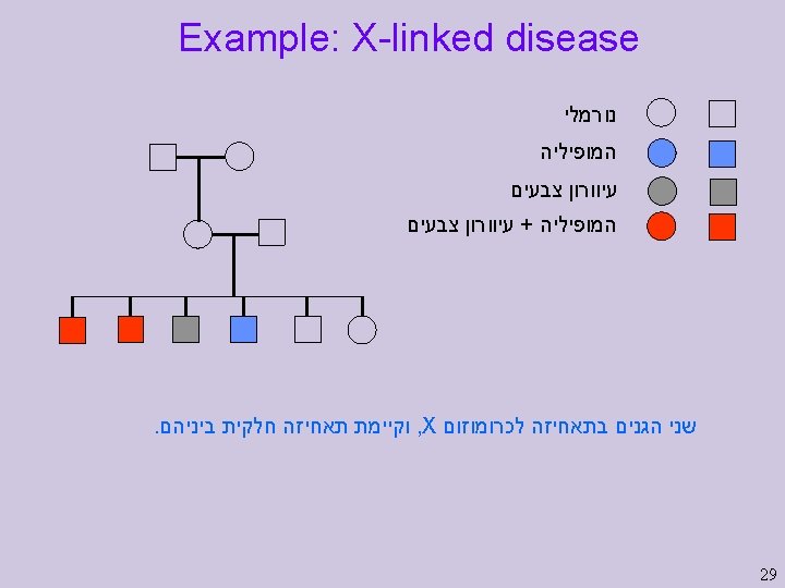
Example: Y-linked disease 28

The population matters History: pattern of growth, immigration Composition: homogeneous or melting pot, or in between Mating patterns: family sizes, mate choice Frequencies of disease-related alleles, and of marker alleles Ages of disease-related alleles 30

Bottleneck Effects 106 years 105 years 31

Complex traits Definition vague, but usually thought of as having multiple, possibly interacting loci, with unknown penetrances; and phenocopies. Affected only methods are widely used. The jury is still out on which, if any will succeed. Few success stories so far. Important: heart disease, cancer susceptibility, diabetes, …are all “complex” traits. We focus more on simple traits where success has been demonstrated very often. About 6 -8 percent of human diseases are thought o be simple Mendelian diseases. 32

Design of gene mapping studies How good are your data implying a genetic component to your trait? Can you estimate the size of the genetic component? Have you got, or will you eventually have enough of the right sort of data to have a good chance of getting a definitive result? Power studies. Simulations. 33

Genotyping A person is said to be typed if its markers have been genotyped. Choice of markers: highly polymorphic preferred. Heterozygosity and polymorphism information content (PIC) value are measures commonly used. Reliability of markers important too Good quality data critical: errors can play a surprisingly large role. 34

Preparing genotype data for analysis Data cleaning is the big issue here. Need much ancillary data…how good is it? 35

Analysis A very large range of methods/programs are available. Effort to understand their theory will pay off in leading to the right choice of analysis tools. Trying everything is not recommended, but not uncommon. Many opportunities for innovation. 36

Interpretation of results of analysis An important issue here is whether you have established linkage. The standards seem to be getting increasingly stringent. What p-value or LOD should you use? Dealing with multiple testing, especially in the context of genome scans and the use of multiple models and multiple phenotypes, is one of the big issues. 37

Replication of results This has recently become a big issue with complex diseases, especially in psychiatry. Nature Genetics suggested in May 1998 that they will require replication before publishing results mapping complex traits. Simulations by Suarez et al (1994) show that sample sizes necessary for replication may be substantially greater than that needed for first detection. 38

Topics not mentioned Exclusion mapping, homozygosity mapping, interference, variance component methods, twin studies, and much more. Some of these topics plus others are covered in two books: Handbook of Human Genetic Linkage by J. D. Terwilliger & J. Ott (1994) Johns Hopkins University Press. Ordered, not available at the library. Analysis of Human Genetic Linkage by J. Ott, 3 rd Edition (1999), Johns Hopkins University Press. 39
 event of interest occurs with rate (per length")
The Poisson Distribution Suppose a (rare) event of interest occurs with rate (per length or time units). For example number of dead birds along a highway. Number of births in one hour. Or the number of crossovers along a chromosome. If we assume that: 1. For an arbitrarily small unit of distance (time) the probability of observing an event is approximately equal to , and equals virtually zero for more than one event. 2. The rate is constant over the entire region. 3. The number of events occurring in one interval is independent of the number of events occurring in a previous disjoint interval, then, the probability for the number of events I occurring at an interval of length t is the Poisson distribution given by: 40
. f(0)")
A mapping function =Expected number of crossovers in a unit distance (1000 bp). f(0) = e- t = the probability of no crossovers in t distance units. RF = 0. 5(1 - e- t ) Because recombinant occur only if crossovers are present, and in that case, half gametes are recombinants and half are not. Note that RF < 0. 5 This relates a genetic distance (RF) with a physical distance t. 41
- Slides: 41