Introduction to GAMS Water Resources Planning and Management

Introduction to GAMS Water Resources Planning and Management Daene C. Mc. Kinney

Introduction To GAMS • GAMS = General Algebraic Modeling System • GAMS Guide and Tutorials – http: //gams. com/docs/document. htm Doc’s here • GAMS website – www. gams. com – http: //gams. com/download/ Download here • Mc. Kinney and Savitsky Tutorials – http: //www. caee. utexas. edu/prof/mckinney/ce 385 d/Lectures/ Mc. Kinney_and_Savitsky. pdf Doc’s here

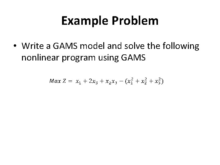
Example Problem • Write a GAMS model and solve the following nonlinear program using GAMS

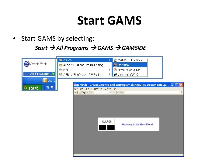
Start GAMS • Start GAMS by selecting: Start All Programs GAMSIDE

Create New GAMS Project • Choose from the GAMSIDE: File Project New project

Name New GAMS Project • In “My Documents” • Create a new directory by pressing the “folder” icon. • Name the new folder “Example” • Double click on “Example” folder • Type “Eq 1” in the “File Name” box • Press Open

New Project • The GAMS window should now show the new Eq 1. gpr project window

Create New GAMS Code File • Select: File New • You should see the new file “Untitled_1. gms”

Enter GAMS Code • The Model • The code VARIABLES Z, X 1, X 2, X 3; Define Variables EQUATIONS F ; F. . Z =E= X 1+2*X 3+X 2*X 3 -X 1*X 1 -X 2*X 2 -X 3*X 3 ; Define Equations MODEL HW 41 /ALL/; Define Model SOLVE HW 41 USING NLP MAXIMIZING Z; Solve Model FILE res /HW 41. txt/; PUT res; put "Solution X 1 = ", put X 1. L, put /; put " X 2 = ", put X 2. L, put /; put " X 3 = ", put X 3. L, put /; Write Output

Enter GAMS Code • The Model • The code

Run the Model • Select: File Run, or Press the red arrow button

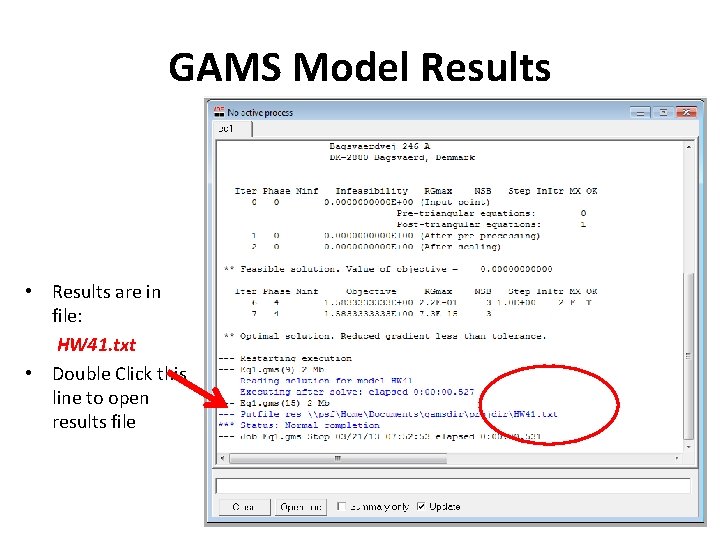
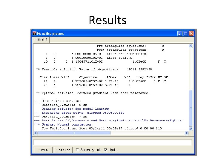
GAMS Model Results • Results are in file: HW 41. txt • Double Click this line to open results file

Viewing Results File • Note Tabs • Results

Another Example Model How to determine the coefficients: Least Squares Regression Residual Model Observation

Observations t 1 2 3 4 5 6 7 8 x 1(t) 2 3 3 3 5 5 6 7 x 2(t) 30 60 70 60 80 90 100 x 3(t) 1 6 7 3 5 9 8 17 y(t) 10 20 30 20 40 50 60 70

Second GAMS Code Define Sets & Data Define Variables Define Equations Define & Solve Model Write Output

Results

Results 80 70 60 y 50 40 y(t)_hat 30 y(t) 20 10 0 0 2 4 time, t 6 8 10

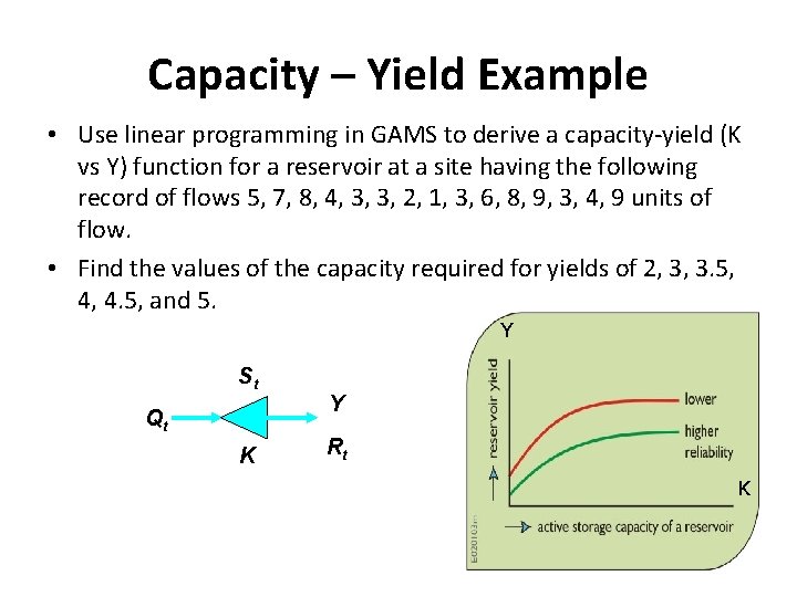
Capacity – Yield Example • Use linear programming in GAMS to derive a capacity-yield (K vs Y) function for a reservoir at a site having the following record of flows 5, 7, 8, 4, 3, 3, 2, 1, 3, 6, 8, 9, 3, 4, 9 units of flow. • Find the values of the capacity required for yields of 2, 3, 3. 5, 4, 4. 5, and 5. Y St Qt K Y Rt K

Capacity – Yield Curve St Qt K Y Rt Y K

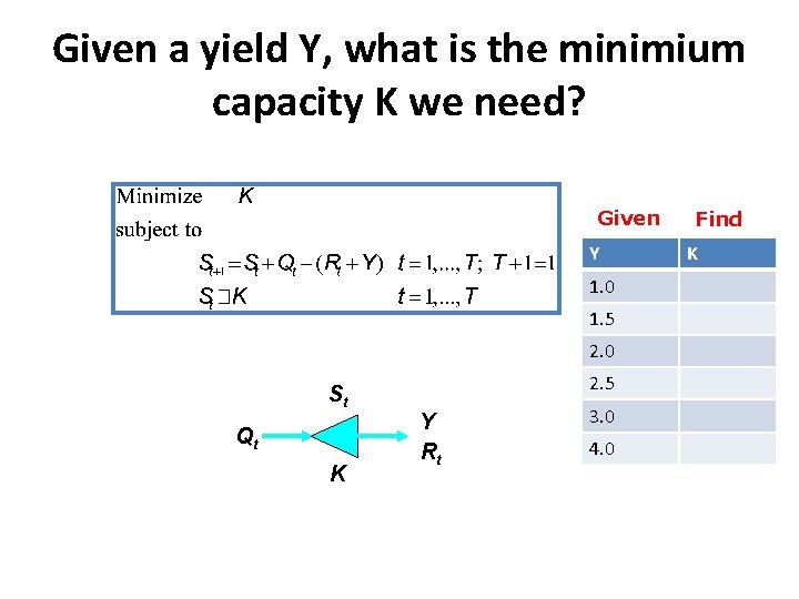
Given a yield Y, what is the minimium capacity K we need? Given Y 1. 0 1. 5 2. 0 St Qt K 2. 5 Y Rt 3. 0 4. 0 Find K

The GAMS Code

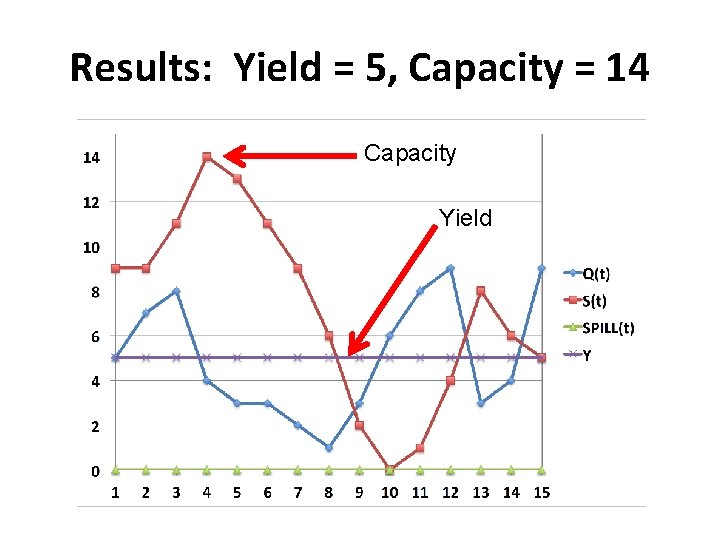
Results: Yield = 5, Capacity = 14

Results: Yield = 5, Capacity = 14 Capacity Yield

Capacity vs Yield Curve

The DOLLAR Sign S(t+1)$(ord(t) lt 15) + S('1')$(ord(t) eq 15) =e= S(t) + Q(t)- SPILL(t) - Y; you can exclude part of an equation by using logical conditions ($ operator) in the name of an equation or in the computation part of an equation. The ORD operator returns an ordinal number equal to the index position in a set.

Management of a Single Reservoir • 2 common tasks of reservoir modeling: 1. Determine coefficients of functions that describe reservoir characteristics 2. Determine optimal mode of reservoir operation (storage volumes, elevations and releases) while satisfying downstream water demands

Reservoir Operation • Compute optimal operation of reservoir given a series of inflows and downstream water demands where: St St-1 Qt Rt Dt K Smin End storage period t, (L 3); Beginning storage period t, (L 3); Inflow period t, (L 3); Release period t, (L 3); Demand, (L 3); and Capacity, (L 3) Dead storage, (L 3)

Comparison of Average and Dry Conditions

GAMS Code SCALAR K /19500/; SCALAR S_min /5500/; SCALAR beg_S /15000/; Capacity Dead storage Beginning storage SETS t / t 1*t 12/; These $include statements allow Us to read in lines from other files: Flows (Q) Demands (D) Evaporation (at, bt) $include River 1 B_Q_Dry. inc $include River 1 B_D. inc $include River 1 B_Evap. inc VARIABLES obj; POSITIVE VARIABLES S(t), R(t); S. UP(t)=K; S. LO(t)=S_min; Set bounds on: Capacity Dead storage

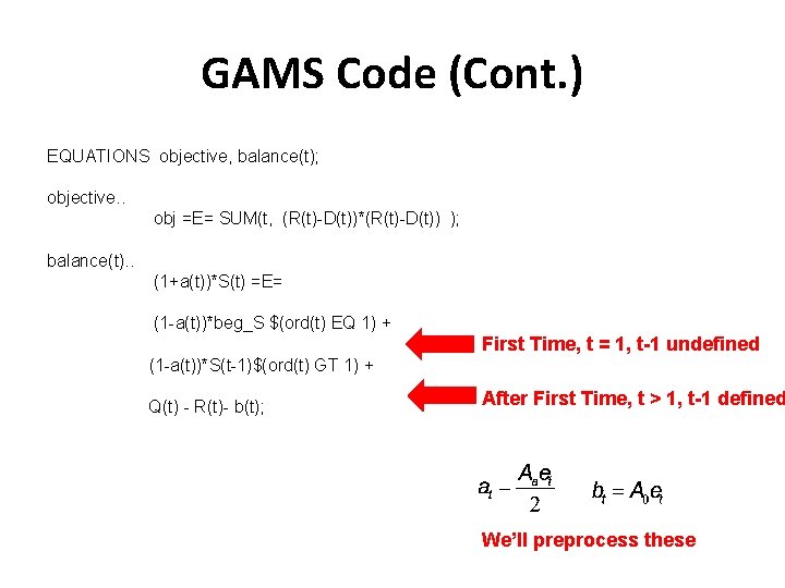
GAMS Code (Cont. ) EQUATIONS objective, balance(t); objective. . obj =E= SUM(t, (R(t)-D(t))*(R(t)-D(t)) ); balance(t). . (1+a(t))*S(t) =E= (1 -a(t))*beg_S $(ord(t) EQ 1) + First Time, t = 1, t-1 undefined (1 -a(t))*S(t-1)$(ord(t) GT 1) + Q(t) - R(t)- b(t); After First Time, t > 1, t-1 defined We’ll preprocess these

$include Files Flows (Q) Demands (D) Evaporation (at, bt) Parameter Q(t) inflow (million m 3) * dry / t 1 375 t 2 361 t 3 448 t 4 518 t 5 1696 t 6 2246 t 7 2155 t 8 1552 t 9 756 t 10 531 t 11 438 t 12 343 /; Parameter D(t) demand (million m 3) / t 1 1699. 5 t 2 1388. 2 t 3 1477. 6 t 4 1109. 4 t 5 594. 6 t 6 636. 6 t 7 1126. 1 t 8 1092. 0 t 9 510. 8 t 10 868. 5 t 11 1049. 8 t 12 1475. 5 /; Parameter a(t) evaporation coefficient / t 1 0. 000046044 t 2 0. 00007674 … t 11 0. 000103599 t 12 0. 000053718/; Parameter b(t) evaporation coefficient / t 1 1. 92 t 2 3. 2 … t 11 4. 32 t 12 2. 24/;

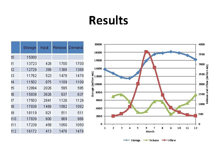
Results Input 20000 Release Demand 4000 18000 t 0 15000 t 1 13723 426 1700 3500 16000 1700 3000 14000 12729 399 1388 t 3 11762 523 1478 t 4 11502 875 1109 t 5 12894 2026 595 t 6 15838 3626 637 t 7 17503 2841 1126 6000 t 8 17838 1469 1092 4000 t 9 18119 821 511 t 10 17839 600 869 t 11 17239 458 1050 t 12 16172 413 1476 Storage (million m 3) t 2 2500 12000 10000 2000 8000 1500 1000 500 2000 0 0 1 2 3 4 5 Storage 6 7 Month Release 8 9 Inflow 10 11 12 Release and Inflow (million m 3) Storage