Introduction to fractional Brownian Motion for Terrain CS

Introduction to fractional Brownian Motion for Terrain CS 658

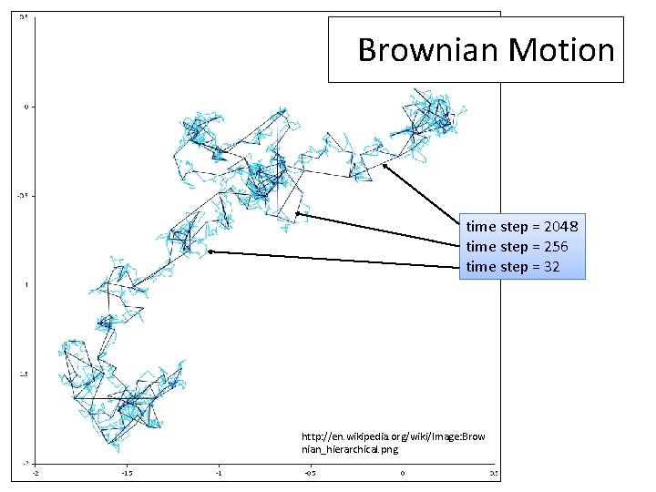
Brownian Motion time step = 2048 time step = 256 time step = 32 http: //en. wikipedia. org/wiki/Image: Brow nian_hierarchical. png

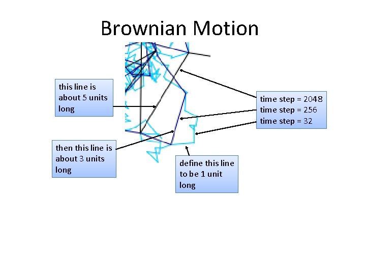
Brownian Motion this line is about 5 units long then this line is about 3 units long time step = 2048 time step = 256 time step = 32 define this line to be 1 unit long

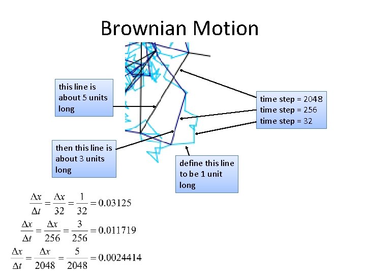
Brownian Motion this line is about 5 units long then this line is about 3 units long time step = 2048 time step = 256 time step = 32 define this line to be 1 unit long

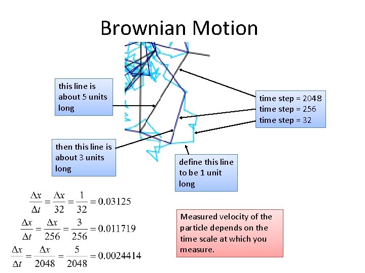
Brownian Motion this line is about 5 units long then this line is about 3 units long time step = 2048 time step = 256 time step = 32 define this line to be 1 unit long Measured velocity of the particle depends on the time scale at which you measure.

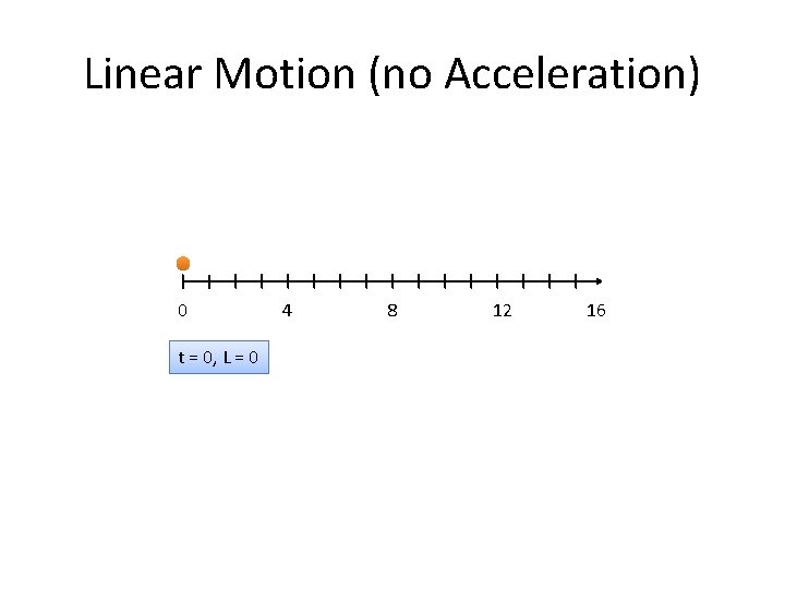
Linear Motion (no Acceleration) 0 t = 0, L = 0 4 8 12 16

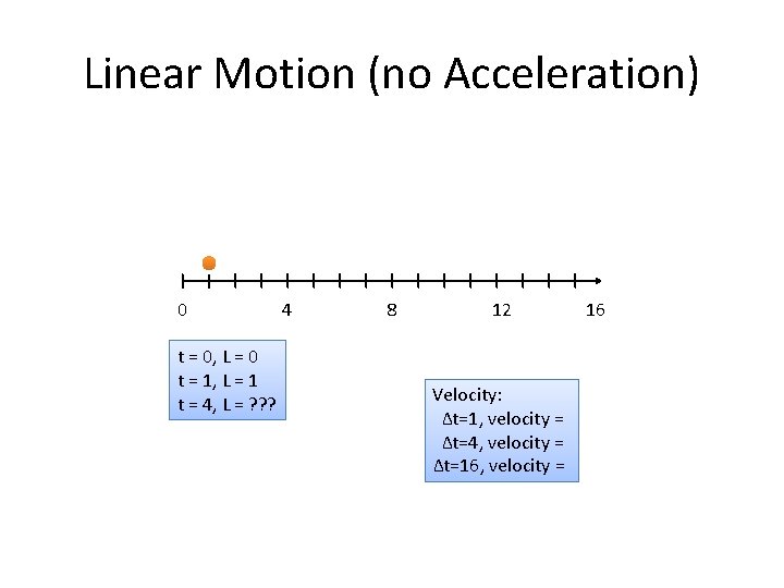
Linear Motion (no Acceleration) 0 t = 0, L = 0 t = 1, L = 1 t = 4, L = ? ? ? 4 8 12 Velocity: Δt=1, velocity = Δt=4, velocity = Δt=16, velocity = 16

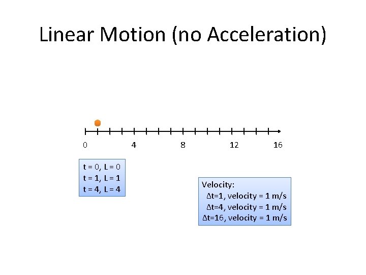
Linear Motion (no Acceleration) 0 t = 0, L = 0 t = 1, L = 1 t = 4, L = 4 4 8 12 16 Velocity: Δt=1, velocity = 1 m/s Δt=4, velocity = 1 m/s Δt=16, velocity = 1 m/s

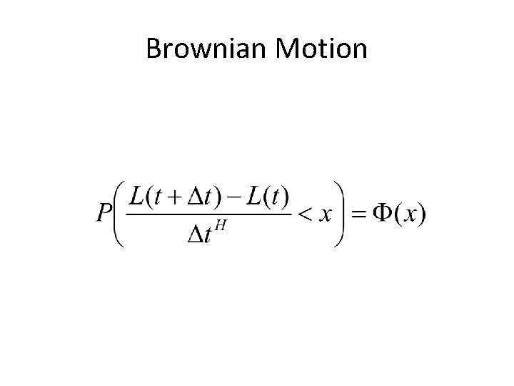
Brownian Motion

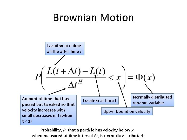
Brownian Motion Location at a time a little after time t Amount of time that has passed but tweaked so that velocity increases with small decreases in t (when t < 1) Location at time t Normally distributed random variable. Upper bound on velocity Probability, P, that a particle has velocity below x, when measured at time interval ∆t, is normally distributed.

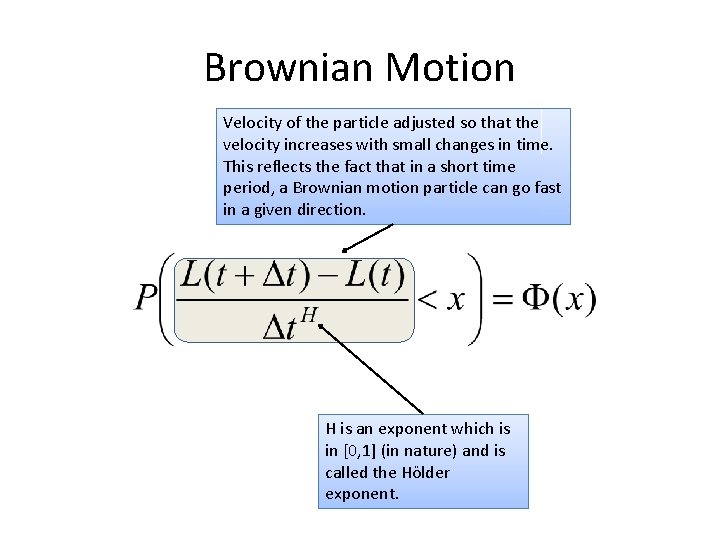
Brownian Motion Velocity of the particle adjusted so that the velocity increases with small changes in time. This reflects the fact that in a short time period, a Brownian motion particle can go fast in a given direction. H is an exponent which is in [0, 1] (in nature) and is called the Hölder exponent.

Brownian Motion this line is about 5 units long then this line is about 3 units long time step = 2048 time step = 256 time step = 32 define this line to be 1 unit long

Brownian Motion in the Frequency Domain • Look at 1 D Brownian motion… http: //www. stat. umn. edu/~charlie/Stoch/brown. html

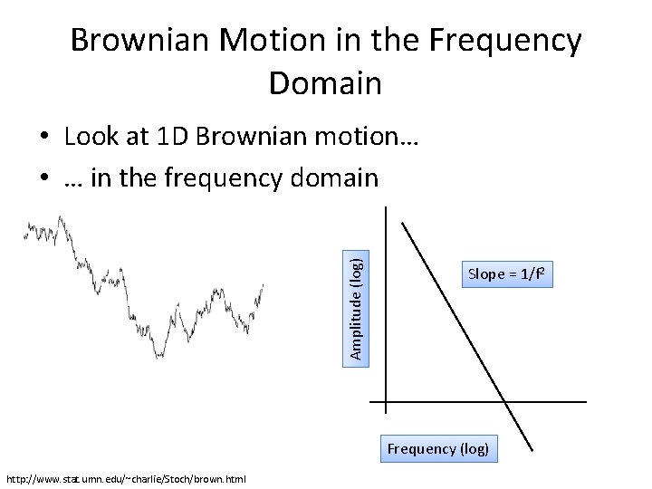
Brownian Motion in the Frequency Domain Amplitude (log) • Look at 1 D Brownian motion… • … in the frequency domain • Slope = 1/f 2 Frequency (log) http: //www. stat. umn. edu/~charlie/Stoch/brown. html

Amplitude (log) Brownian Motion in the Frequency Domain Slope = 1/f 2 Frequency (log) This, by the way, is called “Brown noise” http: //www. stat. umn. edu/~charlie/Stoch/brown. html

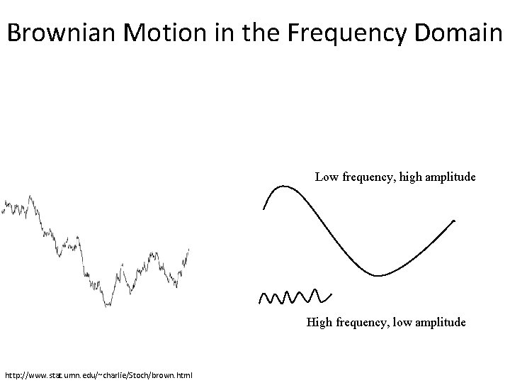
Brownian Motion in the Frequency Domain Low frequency, high amplitude High frequency, low amplitude http: //www. stat. umn. edu/~charlie/Stoch/brown. html

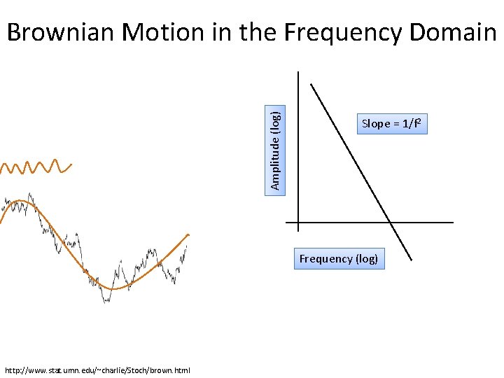
Amplitude (log) Brownian Motion in the Frequency Domain Slope = 1/f 2 Frequency (log) http: //www. stat. umn. edu/~charlie/Stoch/brown. html

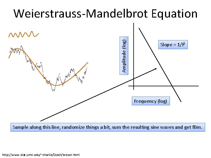
Amplitude (log) Weierstrauss-Mandelbrot Equation Slope = 1/f 2 Frequency (log) Sample along this line, randomize things a bit, sum the resulting sine waves and get f. Bm. http: //www. stat. umn. edu/~charlie/Stoch/brown. html

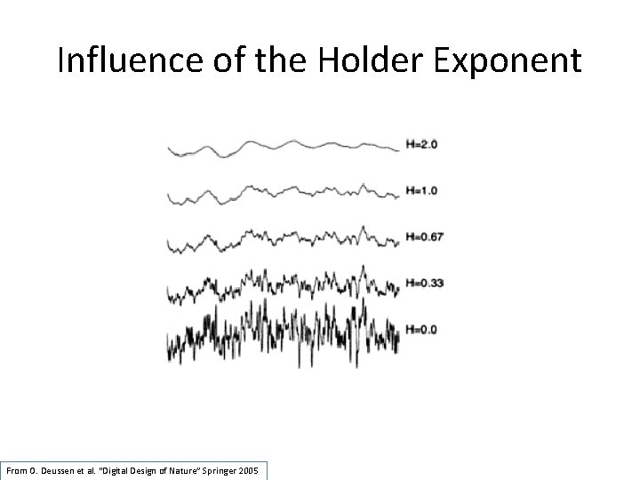
Influence of the Holder Exponent From O. Deussen et al. “Digital Design of Nature” Springer 2005

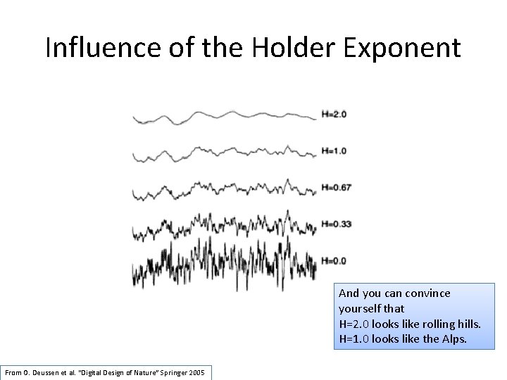
Influence of the Holder Exponent And you can convince yourself that H=2. 0 looks like rolling hills. H=1. 0 looks like the Alps. From O. Deussen et al. “Digital Design of Nature” Springer 2005

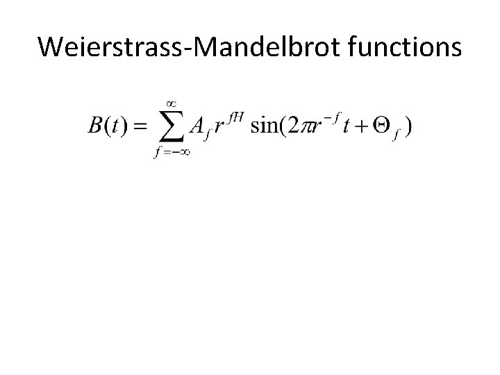
Weierstrass-Mandelbrot functions

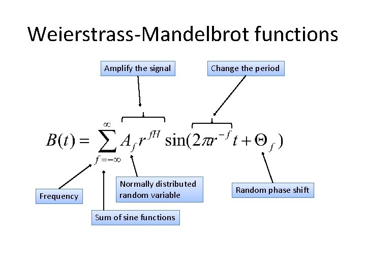
Weierstrass-Mandelbrot functions Amplify the signal Frequency Normally distributed random variable Sum of sine functions Change the period Random phase shift