Introduction to FORTRAN Serial programming A simple example

Introduction to FORTRAN Serial programming

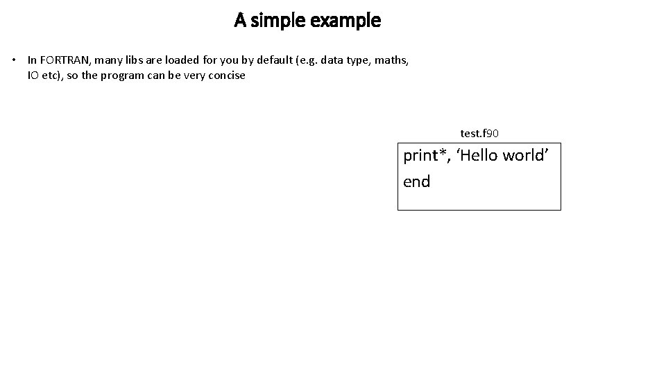
A simple example • In FORTRAN, many libs are loaded for you by default (e. g. data type, maths, IO etc), so the program can be very concise test. f 90 print*, ‘Hello world’ end

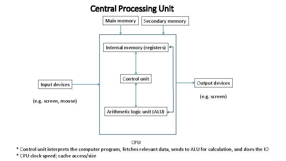
Central Processing Unit Main memory Secondary memory Internal memory (registers) Input devices Control unit Output devices (e. g. screen) (e. g. screen, mouse) Arithmetic logic unit (ALU) CPU * Control unit interprets the computer program, fetches relevant data, sends to ALU for calculation, and does the IO * CPU clock speed; cache access/size

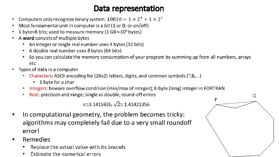
Data representation P • • In computational geometry, the problem becomes tricky: algorithms may completely fail due to a very small roundoff error! Remedies • Replace the actual value with its bounds • Estimate the numerical errors Q

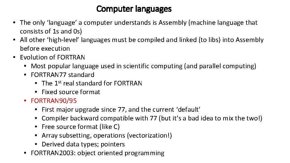
Computer languages • The only ‘language’ a computer understands is Assembly (machine language that consists of 1 s and 0 s) • All other ‘high-level’ languages must be compiled and linked (to libs) into Assembly before execution • Evolution of FORTRAN • Most popular language used in scientific computing (and parallel computing) • FORTRAN 77 standard • The 1 st real standard for FORTRAN • Fixed source format • FORTRAN 90/95 • First major upgrade since 77, and the current ‘default’ • Compiler backward compatible with 77 (but it’s a bad idea to mix the two!) • Free source format (like C) • Array subsetting, operations (vectorization!) • Derived data types; pointers • FORTRAN 2003: object oriented programming

3 D modeling D eliberation: good planning is key D iscipline: follow thru with a well defined plan methodically; resist distractions D illigence: work hard and get used to multi-tasking; attention to details Computers do not lie (well, unless you teeter around the machine precision)

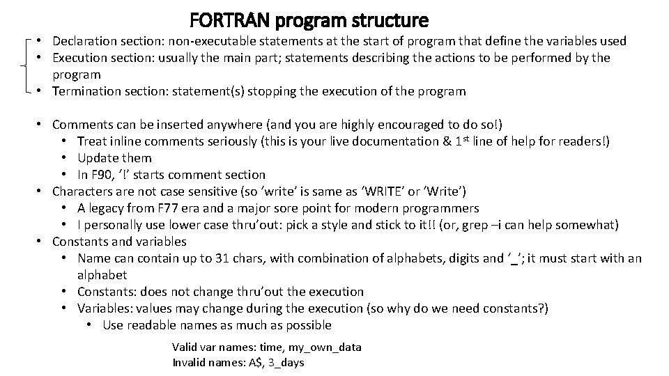
FORTRAN program structure • Declaration section: non-executable statements at the start of program that define the variables used • Execution section: usually the main part; statements describing the actions to be performed by the program • Termination section: statement(s) stopping the execution of the program • Comments can be inserted anywhere (and you are highly encouraged to do so!) • Treat inline comments seriously (this is your live documentation & 1 st line of help for readers!) • Update them • In F 90, ‘!’ starts comment section • Characters are not case sensitive (so ‘write’ is same as ‘WRITE’ or ‘Write’) • A legacy from F 77 era and a major sore point for modern programmers • I personally use lower case thru’out: pick a style and stick to it!! (or, grep –i can help somewhat) • Constants and variables • Name can contain up to 31 chars, with combination of alphabets, digits and ‘_’; it must start with an alphabet • Constants: does not change thru’out the execution • Variables: values may change during the execution (so why do we need constants? ) • Use readable names as much as possible Valid var names: time, my_own_data Invalid names: A$, 3_days

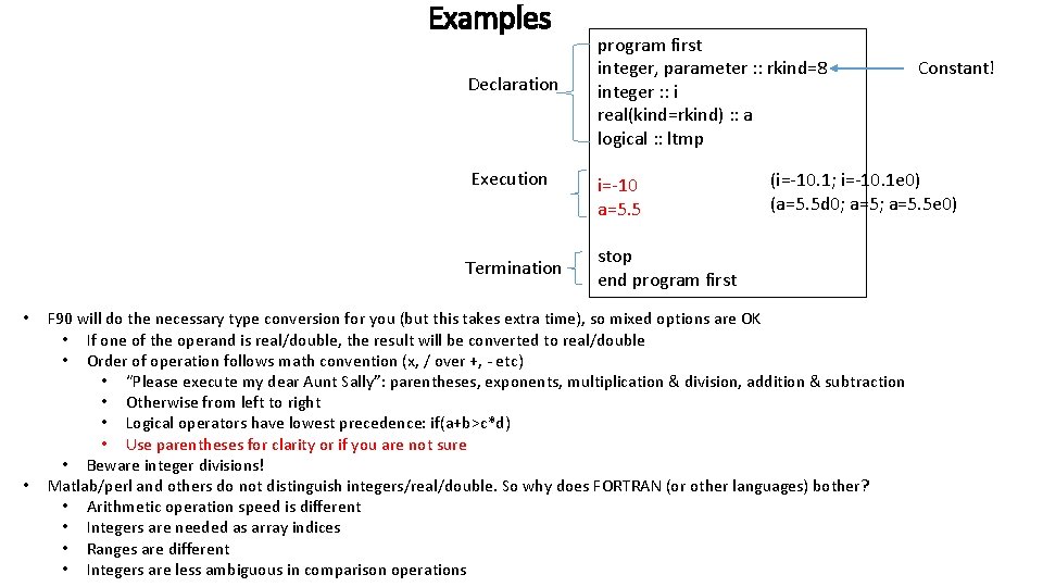
Examples Declaration Execution Termination • • program first integer, parameter : : rkind=8 integer : : i real(kind=rkind) : : a logical : : ltmp i=-10 a=5. 5 Constant! (i=-10. 1; i=-10. 1 e 0) (a=5. 5 d 0; a=5. 5 e 0) stop end program first F 90 will do the necessary type conversion for you (but this takes extra time), so mixed options are OK • If one of the operand is real/double, the result will be converted to real/double • Order of operation follows math convention (x, / over +, - etc) • “Please execute my dear Aunt Sally”: parentheses, exponents, multiplication & division, addition & subtraction • Otherwise from left to right • Logical operators have lowest precedence: if(a+b>c*d) • Use parentheses for clarity or if you are not sure • Beware integer divisions! Matlab/perl and others do not distinguish integers/real/double. So why does FORTRAN (or other languages) bother? • Arithmetic operation speed is different • Integers are needed as array indices • Ranges are different • Integers are less ambiguous in comparison operations

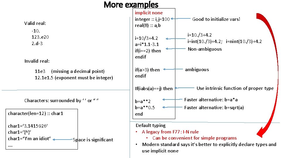
More examples implicit none integer : : i, j=100 real(8) : : a, b Valid real: -10. 123. e 20 2. d-3 i=10/3+4. 2 a=i*1. 1 -3. 1 if(i==2) then endif Invalid real: 11 e 3 (missing a decimal point) 12. 1 e 1. 5 (exponent must be integer) if(a>3) then endif If(iabs(a)==j) then Characters: surrounded by ‘ ’ or “ ” character(len=12) : : char 1=‘ 3. 1415926’ char 1=‘{^}’ char 1=“I’m an idiot” …. Space is significant b=a**2 b=a**0. 5 end Good to initialize vars! i=10. /3+4. 2 i=int(10. /3)+4. 2; i=nint(10. /3)+4. 2 Non-ambiguous Use intrinsic function of proper type Faster alternative: b=a*a Faster alternative: b=sqrt(a) Default typing • A legacy from F 77: I-N rule • Can be convenient for simple programs • Modern standard says it’s better to explicitly declare types and use implicit none

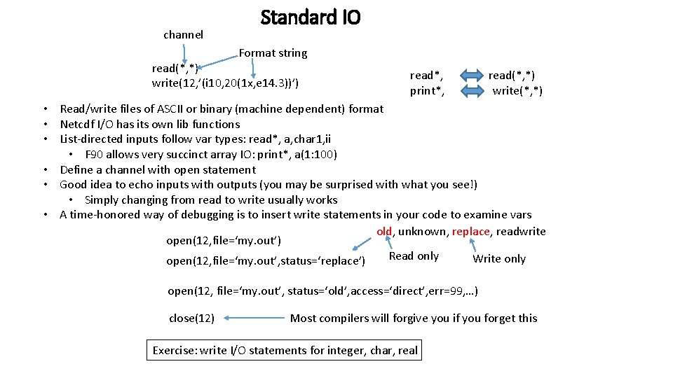
channel Standard IO Format string read(*, *) write(12, ’(i 10, 20(1 x, e 14. 3))’) read*, print*, read(*, *) write(*, *) • Read/write files of ASCII or binary (machine dependent) format • Netcdf I/O has its own lib functions • List-directed inputs follow var types: read*, a, char 1, ii • F 90 allows very succinct array IO: print*, a(1: 100) • Define a channel with open statement • Good idea to echo inputs with outputs (you may be surprised with what you see!) • Simply changing from read to write usually works • A time-honored way of debugging is to insert write statements in your code to examine vars old, unknown, replace, readwrite open(12, file=‘my. out’) Read only Write only open(12, file=‘my. out’, status=‘replace’) open(12, file=‘my. out’, status=‘old’, access=‘direct’, err=99, …) close(12) Most compilers will forgive you if you forget this Exercise: write I/O statements for integer, char, real

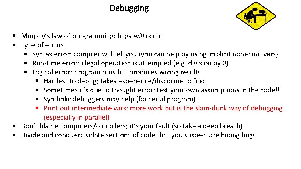
Debugging § Murphy’s law of programming: bugs will occur § Type of errors § Syntax error: compiler will tell you (you can help by using implicit none; init vars) § Run-time error: illegal operation is attempted (e. g. division by 0) § Logical error: program runs but produces wrong results § Hardest to debug; takes experience/discipline to find § Sometimes it’s due to thought error: test your own assumptions in the code!! § Symbolic debuggers may help (for serial program) § Print out intermediate vars: more work but is the slam-dunk way of debugging (especially in parallel) § Don’t blame computers/compilers; it’s your fault (so take a deep breath) § Divide and conquer: isolate sections of code that you suspect are hiding bugs

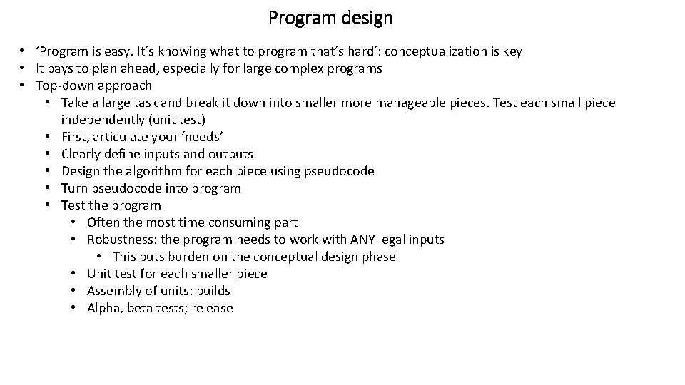
Program design • ‘Program is easy. It’s knowing what to program that’s hard’: conceptualization is key • It pays to plan ahead, especially for large complex programs • Top-down approach • Take a large task and break it down into smaller more manageable pieces. Test each small piece independently (unit test) • First, articulate your ‘needs’ • Clearly define inputs and outputs • Design the algorithm for each piece using pseudocode • Turn pseudocode into program • Test the program • Often the most time consuming part • Robustness: the program needs to work with ANY legal inputs • This puts burden on the conceptual design phase • Unit test for each smaller piece • Assembly of units: builds • Alpha, beta tests; release

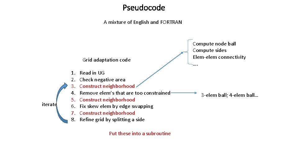
Pseudocode A mixture of English and FORTRAN Grid adaptation code iterate 1. 2. 3. 4. 5. 6. 7. 8. Read in UG Check negative area Construct neighborhood Remove elem’s that are too constrained Construct neighborhood Fix skew elem by edge swapping Construct neighborhood Refine grid by splitting a side Put these into a subroutine Compute node ball Compute sides Elem-elem connectivity …. 3 -elem ball; 4 -elem ball…

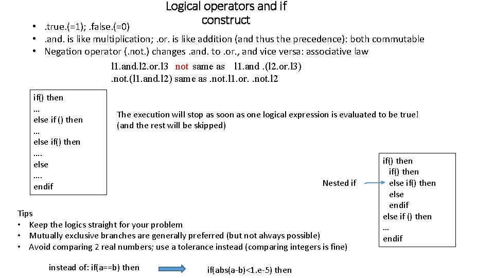
Logical operators and if construct • . true. (=1); . false. (=0) • . and. is like multiplication; . or. is like addition (and thus the precedence): both commutable • Negation operator (. not. ) changes. and. to. or. , and vice versa: associative law l 1. and. l 2. or. l 3 not same as l 1. and. (l 2. or. l 3). not. (l 1. and. l 2) same as. not. l 1. or. . not. l 2 if() then … else if() then …. else …. endif The execution will stop as soon as one logical expression is evaluated to be true! (and the rest will be skipped) Nested if Tips • Keep the logics straight for your problem • Mutually exclusive branches are generally preferred (but not always possible) • Avoid comparing 2 real numbers; use a tolerance instead (comparing integers is fine) instead of: if(a==b) then if(abs(a-b)<1. e-5) then if() then else endif else if () then … endif

Do loop 1 st form [name] do index=istart, iend, increment … enddo [name] • index, istart, iend, increment are all integer (expressions). F 90 converts non-integers to integers for you (of course a better way is to use int() explicitly) • index can NOT be changed inside the loop!! • The loop starts with index=istart, and index is incremented by increment each iteration and the loop is terminated when index>iend. The total # of iteration is (iend-istart+ increment)/ increment, so the loop is not executed if # of iteration is <1 (useful for handling of exceptional cases)! • index is undefined after the enddo (and so do NOT use it afterwards!) 2 nd form [name] do …. enddo [name] Also known as do while loop; must have an exit statement to avoid infinite loop • Loop control: cycle (go to next iteration) and exit (jump out of current loop) • ‘name’ is global in scope (i. e. you cannot use same names in different routines; each name must be unique)

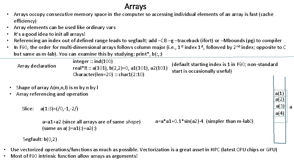
Arrays • Arrays occupy consecutive memory space in the computer so accessing individual elements of an array is fast (cache efficiency) • Array elements can be used like ordinary vars • It’s a good idea to init all arrays! • Referencing an index out of defined range leads to segfault; add –CB –g –traceback (ifort) or –Mbounds (pg) to compiler • In F 90, the order for multi-dimensional arrays follows column major (i. e. , 1 st index 1 st, followed by 2 nd index; opposite to C but same as m-lab). You can examine this by studying: print*, b(: , : ) integer : : ind(100) (default starting index is 1 in F 90; non-standard Array declaration real*8 : : a(101), b(2, 2)=0, a 1(101), a 2(101) start is occasionally useful) Character(len=20) : : char 1(2: 10) • Shape of array A(m, n, l) is m by n by l • Array referencing and operation Slice: a(1) a(2) a(3) a a(4) a(1: 3)=(/0, -1, -2/) a=a 1+a 2 (since all arrays are of same shape) (same as a(: )=a 1(: )+a 2(: ) a=a*a 1+0. 1*sin(a 2)-4 (simpler than m-lab!) Segfault: b(0, 2) • Use vectorized operations/functions as much as possible. Vectorization is a great asset in HPC (latest CPU chips or GPU) • Most of F 90 intrinsic function allow arrays as arguments!

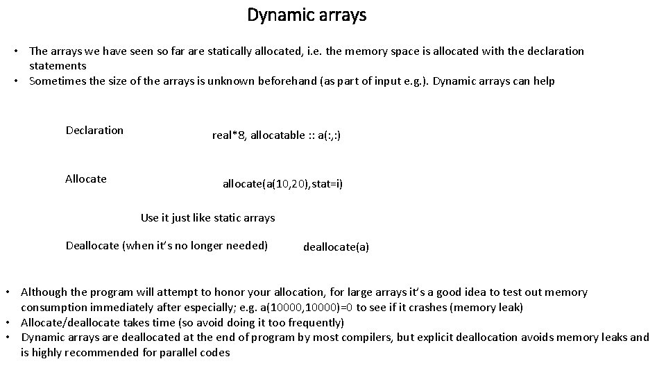
Dynamic arrays • The arrays we have seen so far are statically allocated, i. e. the memory space is allocated with the declaration statements • Sometimes the size of the arrays is unknown beforehand (as part of input e. g. ). Dynamic arrays can help Declaration Allocate real*8, allocatable : : a(: , : ) allocate(a(10, 20), stat=i) Use it just like static arrays Deallocate (when it’s no longer needed) deallocate(a) • Although the program will attempt to honor your allocation, for large arrays it’s a good idea to test out memory consumption immediately after especially; e. g. a(10000, 10000)=0 to see if it crashes (memory leak) • Allocate/deallocate takes time (so avoid doing it too frequently) • Dynamic arrays are deallocated at the end of program by most compilers, but explicit deallocation avoids memory leaks and is highly recommended for parallel codes

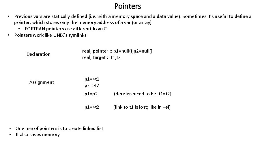
Pointers • Previous vars are statically defined (i. e. with a memory space and a data value). Sometimes it’s useful to define a pointer, which stores only the memory address of a var (or array) • FORTRAN pointers are different from C • Pointers work like UNIX’s symlinks Declaration Assignment real, pointer : : p 1=null(), p 2=null() real, target : : t 1, t 2 p 1=>t 1 p 2=>t 2 p 1=p 2 (dereferenced to be: t 1=t 2) p 1=>t 2 (link to t 1 is lost; like ln –sf) • One use of pointers is to create linked list • It also saves memory

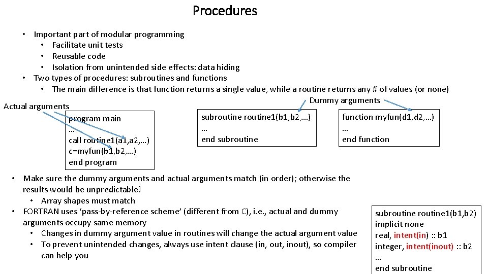
Procedures • Important part of modular programming • Facilitate unit tests • Reusable code • Isolation from unintended side effects: data hiding • Two types of procedures: subroutines and functions • The main difference is that function returns a single value, while a routine returns any # of values (or none) Dummy arguments Actual arguments subroutine 1(b 1, b 2, …) function myfun(d 1, d 2, …) program main … … … end subroutine end function call routine 1(a 1, a 2, …) c=myfun(b 1, b 2, …) end program • Make sure the dummy arguments and actual arguments match (in order); otherwise the results would be unpredictable! • Array shapes must match • FORTRAN uses ‘pass-by-reference scheme’ (different from C), i. e. , actual and dummy arguments occupy same memory • Changes in dummy argument value in routines will change the actual argument value • To prevent unintended changes, always use intent clause (in, out, inout), so compiler can help you subroutine 1(b 1, b 2) implicit none real, intent(in) : : b 1 integer, intent(inout) : : b 2 … end subroutine

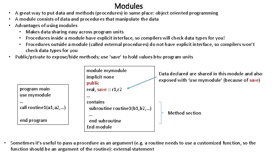
Modules • A great way to put data and methods (procedures) in same place: object oriented programming • A module consists of data and procedures that manipulate the data • Advantages of using modules • Makes data sharing easy across program units • Procedures inside a module have explicit interface, so compilers will check data types for you! • Procedures outside a module (called external procedures) do not have explicit interface, so compilers won’t check data types for you • Public/private to expose/hide methods; use ‘save’ to hold values btw program units program main use mymodule … call routine 1(a 1, a 2, …) end program module mymodule implicit none public real, save : : r 1, r 2 … contains subroutine 1(b 1, b 2, …) … end subroutine End module Data declared are shared in this module and also exposed with ‘use mymodule’ (because of save) Method section • Sometimes it’s useful to pass a procedure as an argument (e. g. a routine needs to use a customized function, so the function should be an argument of the routine): external statement

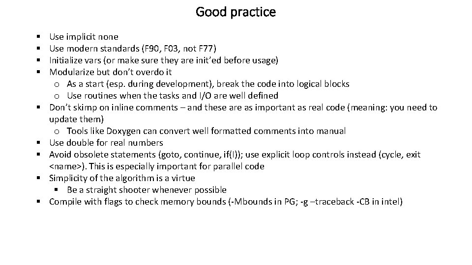
Good practice § § § § § Use implicit none Use modern standards (F 90, F 03, not F 77) Initialize vars (or make sure they are init’ed before usage) Modularize but don’t overdo it o As a start (esp. during development), break the code into logical blocks o Use routines when the tasks and I/O are well defined Don’t skimp on inline comments – and these are as important as real code (meaning: you need to update them) o Tools like Doxygen can convert well formatted comments into manual Use double for real numbers Avoid obsolete statements (goto, continue, if(I)); use explicit loop controls instead (cycle, exit <name>). This is especially important for parallel code Simplicity of the algorithm is a virtue § Be a straight shooter whenever possible Compile with flags to check memory bounds (-Mbounds in PG; -g –traceback -CB in intel)

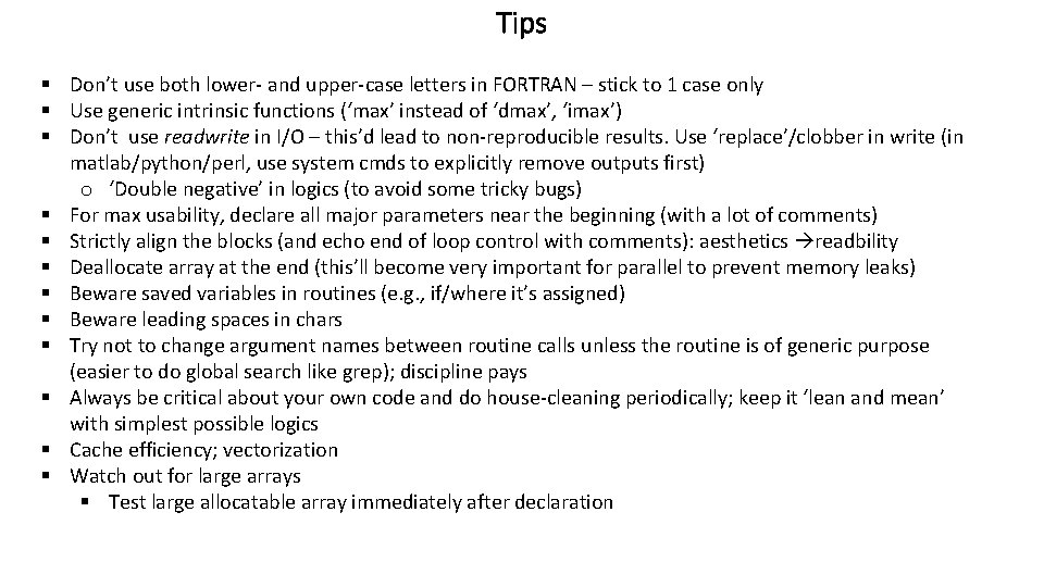
Tips § Don’t use both lower- and upper-case letters in FORTRAN – stick to 1 case only § Use generic intrinsic functions (‘max’ instead of ‘dmax’, ‘imax’) § Don’t use readwrite in I/O – this’d lead to non-reproducible results. Use ‘replace’/clobber in write (in matlab/python/perl, use system cmds to explicitly remove outputs first) o ‘Double negative’ in logics (to avoid some tricky bugs) § For max usability, declare all major parameters near the beginning (with a lot of comments) § Strictly align the blocks (and echo end of loop control with comments): aesthetics readbility § Deallocate array at the end (this’ll become very important for parallel to prevent memory leaks) § Beware saved variables in routines (e. g. , if/where it’s assigned) § Beware leading spaces in chars § Try not to change argument names between routine calls unless the routine is of generic purpose (easier to do global search like grep); discipline pays § Always be critical about your own code and do house-cleaning periodically; keep it ‘lean and mean’ with simplest possible logics § Cache efficiency; vectorization § Watch out for large arrays § Test large allocatable array immediately after declaration

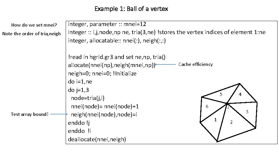
Example 1: Ball of a vertex How do we set mnei? Note the order of tria, neigh Test array bound! integer, parameter : : mnei=12 integer : : i, j, node, np ne, tria(3, ne) !stores the vertex indices of element 1: ne integer, allocatable: : nnei(: ), neigh(: , : ) !read in hgrid. gr 3 and set ne, np, tria() allocate(nnei(np), neigh(mnei, np)) neigh=0; nnei=0; !Initialize do i=1, ne do j=1, 3 node=tria(j, i) nnei(node)= nnei(node)+1 neigh(nnei(node), node)=i enddo !j enddo !i deallocate(nnei, neigh) Cache efficiency 5 6 4 i 1 3 2

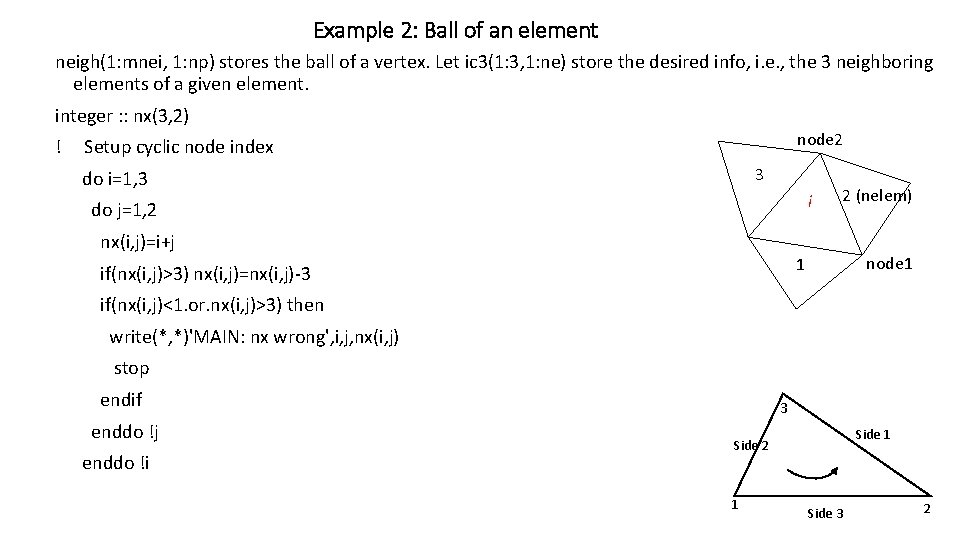
Example 2: Ball of an element neigh(1: mnei, 1: np) stores the ball of a vertex. Let ic 3(1: 3, 1: ne) store the desired info, i. e. , the 3 neighboring elements of a given element. integer : : nx(3, 2) ! node 2 Setup cyclic node index 3 do i=1, 3 i do j=1, 2 nx(i, j)=i+j 2 (nelem) node 1 1 if(nx(i, j)>3) nx(i, j)=nx(i, j)-3 if(nx(i, j)<1. or. nx(i, j)>3) then write(*, *)'MAIN: nx wrong', i, j, nx(i, j) stop endif enddo !j enddo !i 3 Side 1 Side 2 1 Side 3 2

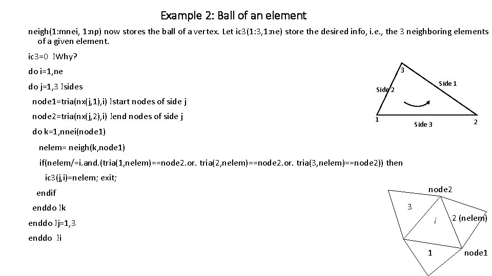
Example 2: Ball of an element neigh(1: mnei, 1: np) now stores the ball of a vertex. Let ic 3(1: 3, 1: ne) store the desired info, i. e. , the 3 neighboring elements of a given element. ic 3=0 !Why? 3 do i=1, ne do j=1, 3 !sides Side 1 Side 2 node 1=tria(nx(j, 1), i) !start nodes of side j node 2=tria(nx(j, 2), i) !end nodes of side j 1 2 Side 3 do k=1, nnei(node 1) nelem= neigh(k, node 1) if(nelem/=i. and. (tria(1, nelem)==node 2. or. tria(2, nelem)==node 2. or. tria(3, nelem)==node 2)) then ic 3(j, i)=nelem; exit; node 2 endif enddo !k 3 i enddo !j=1, 3 2 (nelem) enddo !i 1 node 1

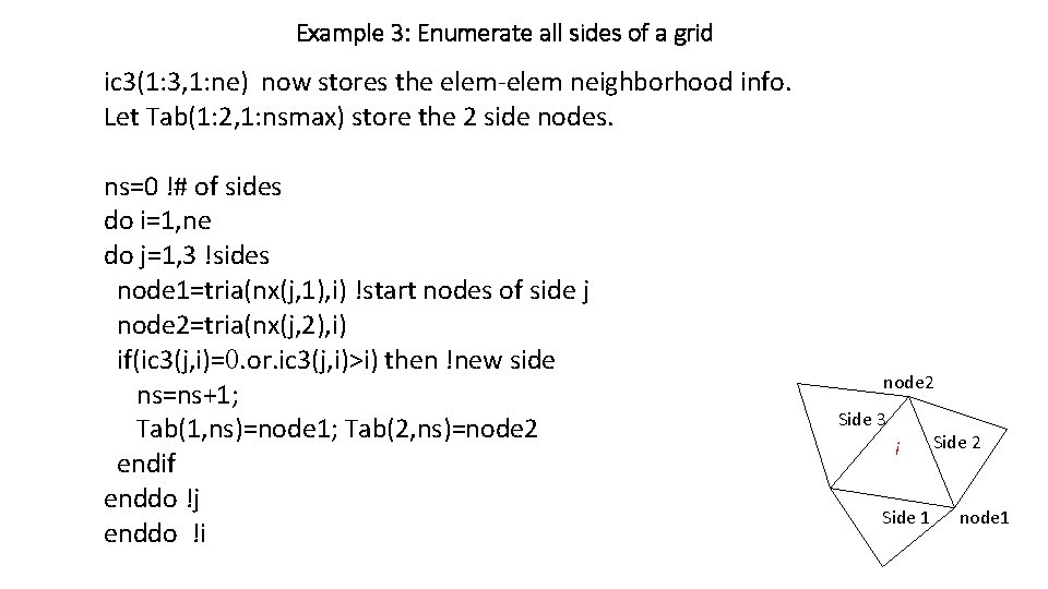
Example 3: Enumerate all sides of a grid ic 3(1: 3, 1: ne) now stores the elem-elem neighborhood info. Let Tab(1: 2, 1: nsmax) store the 2 side nodes. ns=0 !# of sides do i=1, ne do j=1, 3 !sides node 1=tria(nx(j, 1), i) !start nodes of side j node 2=tria(nx(j, 2), i) if(ic 3(j, i)=0. or. ic 3(j, i)>i) then !new side ns=ns+1; Tab(1, ns)=node 1; Tab(2, ns)=node 2 endif enddo !j enddo !i node 2 Side 3 i Side 1 Side 2 node 1

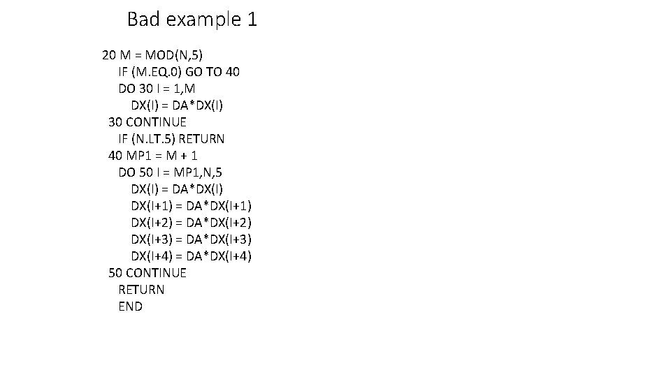
Bad example 1 20 M = MOD(N, 5) IF (M. EQ. 0) GO TO 40 DO 30 I = 1, M DX(I) = DA*DX(I) 30 CONTINUE IF (N. LT. 5) RETURN 40 MP 1 = M + 1 DO 50 I = MP 1, N, 5 DX(I) = DA*DX(I) DX(I+1) = DA*DX(I+1) DX(I+2) = DA*DX(I+2) DX(I+3) = DA*DX(I+3) DX(I+4) = DA*DX(I+4) 50 CONTINUE RETURN END

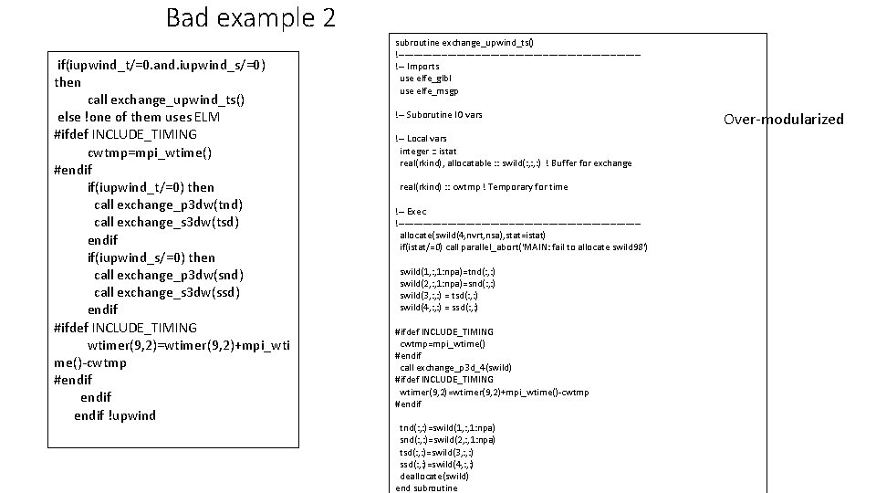
Bad example 2 if(iupwind_t/=0. and. iupwind_s/=0) then call exchange_upwind_ts() else !one of them uses ELM #ifdef INCLUDE_TIMING cwtmp=mpi_wtime() #endif if(iupwind_t/=0) then call exchange_p 3 dw(tnd) call exchange_s 3 dw(tsd) endif if(iupwind_s/=0) then call exchange_p 3 dw(snd) call exchange_s 3 dw(ssd) endif #ifdef INCLUDE_TIMING wtimer(9, 2)=wtimer(9, 2)+mpi_wti me()-cwtmp #endif !upwind subroutine exchange_upwind_ts() !---------------------------------------!-- Imports use elfe_glbl use elfe_msgp !-- Suborutine IO vars !-- Local vars integer : : istat real(rkind), allocatable : : swild(: , : ) ! Buffer for exchange real(rkind) : : cwtmp ! Temporary for time !-- Exec !---------------------------------------allocate(swild(4, nvrt, nsa), stat=istat) if(istat/=0) call parallel_abort('MAIN: fail to allocate swild 98') swild(1, : , 1: npa)=tnd(: , : ) swild(2, : , 1: npa)=snd(: , : ) swild(3, : ) = tsd(: , : ) swild(4, : ) = ssd(: , : ) #ifdef INCLUDE_TIMING cwtmp=mpi_wtime() #endif call exchange_p 3 d_4(swild) #ifdef INCLUDE_TIMING wtimer(9, 2)=wtimer(9, 2)+mpi_wtime()-cwtmp #endif tnd(: , : )=swild(1, : , 1: npa) snd(: , : )=swild(2, : , 1: npa) tsd(: , : )=swild(3, : ) ssd(: , : )=swild(4, : ) deallocate(swild) end subroutine Over-modularized

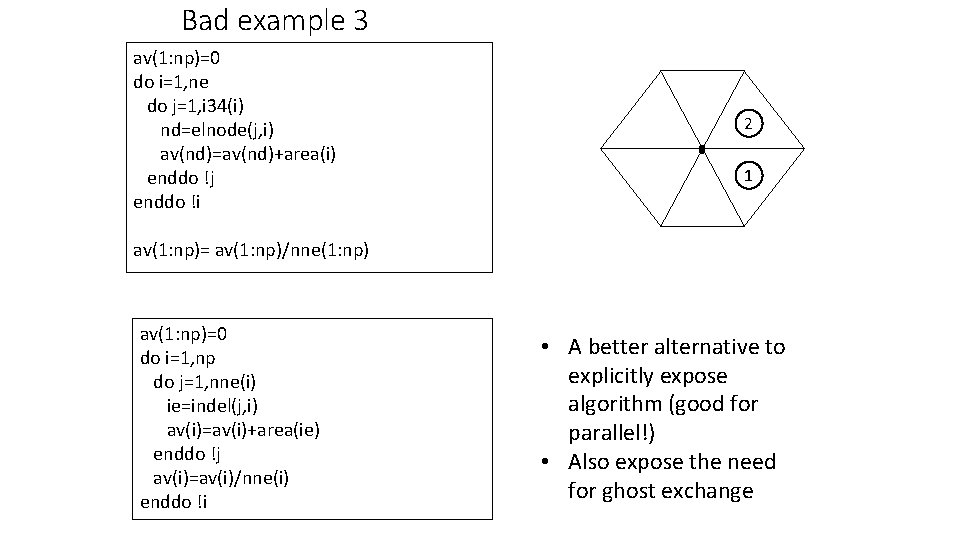
Bad example 3 av(1: np)=0 do i=1, ne do j=1, i 34(i) nd=elnode(j, i) av(nd)=av(nd)+area(i) enddo !j enddo !i 2 1 av(1: np)= av(1: np)/nne(1: np) av(1: np)=0 do i=1, np do j=1, nne(i) ie=indel(j, i) av(i)=av(i)+area(ie) enddo !j av(i)=av(i)/nne(i) enddo !i • A better alternative to explicitly expose algorithm (good for parallel!) • Also expose the need for ghost exchange

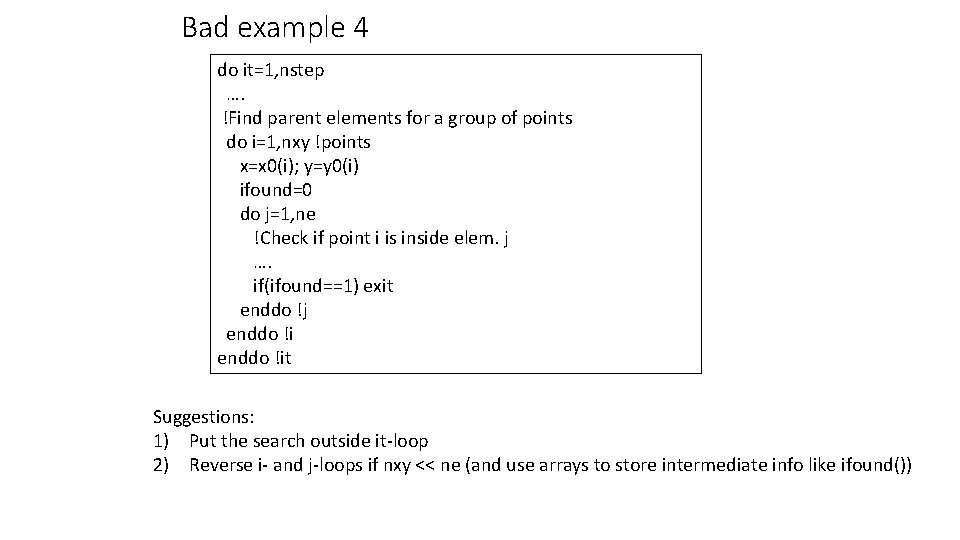
Bad example 4 do it=1, nstep …. !Find parent elements for a group of points do i=1, nxy !points x=x 0(i); y=y 0(i) ifound=0 do j=1, ne !Check if point i is inside elem. j …. if(ifound==1) exit enddo !j enddo !it Suggestions: 1) Put the search outside it-loop 2) Reverse i- and j-loops if nxy << ne (and use arrays to store intermediate info like ifound())

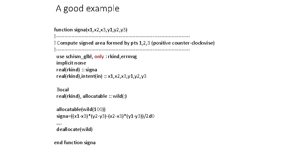
A good example function signa(x 1, x 2, x 3, y 1, y 2, y 3) !---------------------------------------! Compute signed area formed by pts 1, 2, 3 (positive counter-clockwise) !---------------------------------------use schism_glbl, only : rkind, errmsg implicit none real(rkind) : : signa real(rkind), intent(in) : : x 1, x 2, x 3, y 1, y 2, y 3 !local real(rkind), allocatable : : wild(: ) allocatable(wild(100)) signa=((x 1 -x 3)*(y 2 -y 3)-(x 2 -x 3)*(y 1 -y 3))/2 d 0 …. deallocate(wild) end function signa

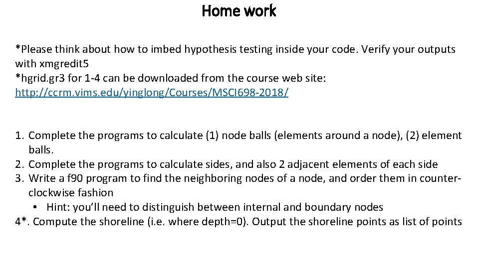
Home work *Please think about how to imbed hypothesis testing inside your code. Verify your outputs with xmgredit 5 *hgrid. gr 3 for 1 -4 can be downloaded from the course web site: http: //ccrm. vims. edu/yinglong/Courses/MSCI 698 -2018/ 1. Complete the programs to calculate (1) node balls (elements around a node), (2) element balls. 2. Complete the programs to calculate sides, and also 2 adjacent elements of each side 3. Write a f 90 program to find the neighboring nodes of a node, and order them in counterclockwise fashion • Hint: you’ll need to distinguish between internal and boundary nodes 4*. Compute the shoreline (i. e. where depth=0). Output the shoreline points as list of points

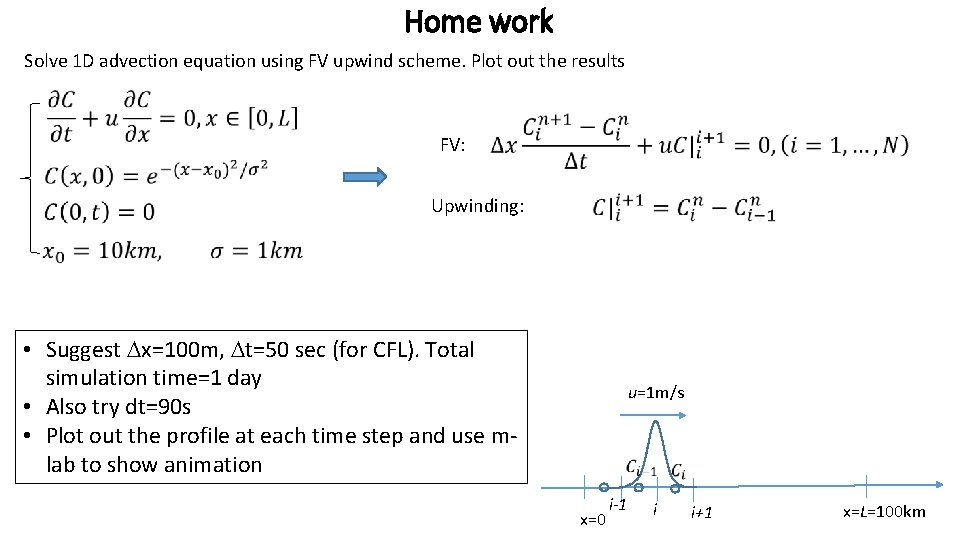
Home work Solve 1 D advection equation using FV upwind scheme. Plot out the results FV: Upwinding: • Suggest Dx=100 m, Dt=50 sec (for CFL). Total simulation time=1 day • Also try dt=90 s • Plot out the profile at each time step and use mlab to show animation u=1 m/s x=0 i-1 i i+1 x=L=100 km