Introduction to Dynamic Programming The sequence alignment problem

Introduction to Dynamic Programming The sequence alignment problem Wilson Leung 08/2015

Outline Overview of the sequence alignment problem Calculate the optimal global alignment Characteristics of dynamic programming algorithms Calculate the optimal local alignment

Learning objectives Understand theory behind sequence alignment Become a better informed user of NCBI BLAST This presentation will not cover: The BLAST algorithm Parameter optimizations Statistics for similarity searches (Karlin-Altschul theory) Korf, I. , Yandell, M. , and Bedell, J. (2003). BLAST. O’Reilly Media, Inc.

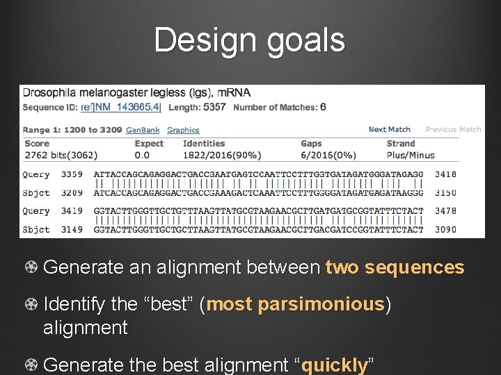
Design goals Generate an alignment between two sequences Identify the “best” (most parsimonious) alignment Generate the best alignment “quickly”

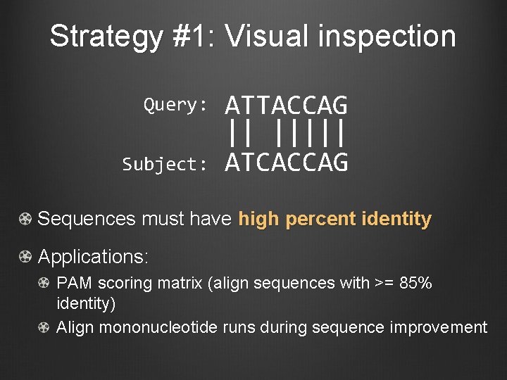
Strategy #1: Visual inspection Query: Subject: ATTACCAG || ||||| ATCACCAG Sequences must have high percent identity Applications: PAM scoring matrix (align sequences with >= 85% identity) Align mononucleotide runs during sequence improvement

Strategy #2: Enumerate all alignments Guaranteed to find the best alignment Does not scale Combinatorial explosion Two 300 bp sequences have ~10179 possible alignments (Eddy 2004) Brute-force algorithm Establish baseline performance and test cases Identify patterns in the problem space

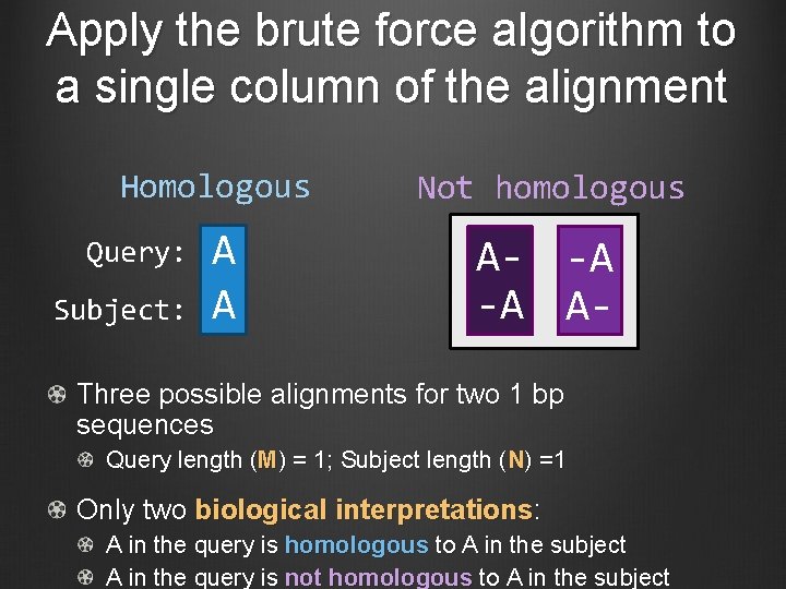
Apply the brute force algorithm to a single column of the alignment Homologous Not homologous A A A- -A -A A- Query: Subject: Three possible alignments for two 1 bp sequences Query length (M) = 1; Subject length (N) =1 Only two biological interpretations: A in the query is homologous to A in the subject A in the query is not homologous to A in the subject

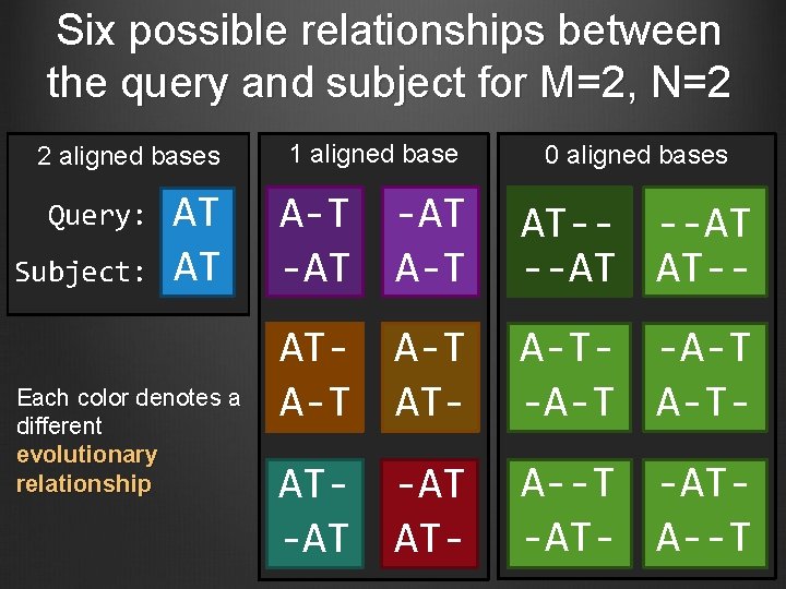
Six possible relationships between the query and subject for M=2, N=2 2 aligned bases Query: Subject: AT AT Each color denotes a different evolutionary relationship 1 aligned base 0 aligned bases A-T -AT A-T AT-- --AT AT-- AT- A-T- -A-T A-T- AT- -AT AT- A--T -AT-AT- A--T

Observations from the brute force alignment strategy Many of the possible alignments are redundant Imply the same evolutionary relationship Large number of possible alignments 13 possible alignments for sequences of length 2 Can ignore many possible alignments Many are suboptimal compared to the best alignment

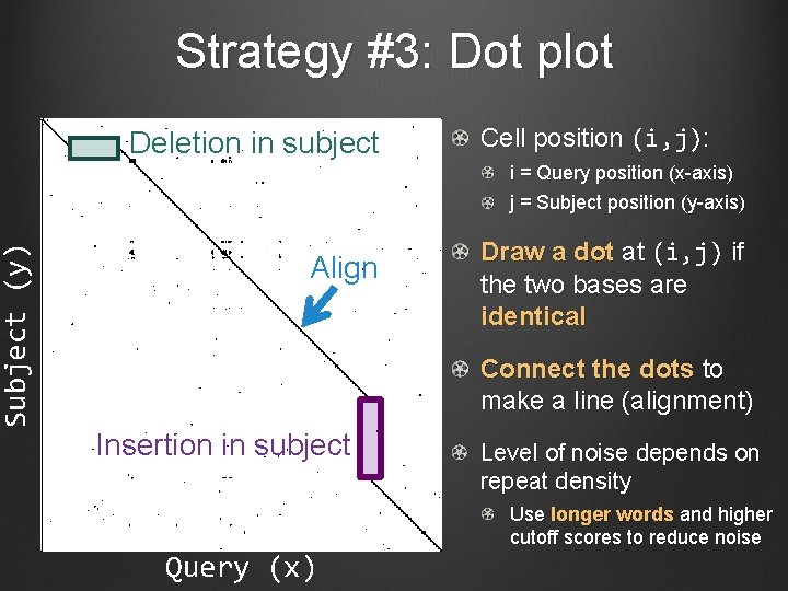
Subject (y) Strategy #3: Dot plot Deletion in subject Cell position (i, j): i = Query position (x-axis) j = Subject position (y-axis) Align Draw a dot at (i, j) if the two bases are identical Connect the dots to make a line (alignment) Insertion in subject Query (x) Level of noise depends on repeat density Use longer words and higher cutoff scores to reduce noise

Assessment of the three sequence alignment strategies Infeasible to examine all possible alignments Need to reduce the search space Only a small subset of alignments are “interesting” Many alignments are redundant Connect the dots in the dot plot to create an alignment Consider the cumulative levels of similarity

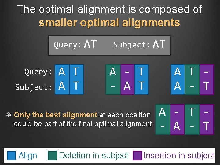
The optimal alignment is composed of smaller optimal alignments Query: AT Query: Subject: A T Subject: AT A - T - A T Only the best alignment at each position could be part of the final optimal alignment Align Deletion in subject A T A - T - A - T Insertion in subject

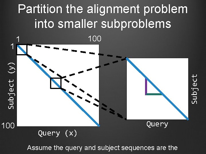
Partition the alignment problem into smaller subproblems 100 Subject (y) 1 100 1 Query (x) Query Assume the query and subject sequences are the

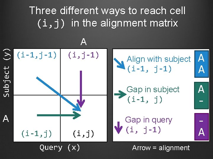
Three different ways to reach cell (i, j) in the alignment matrix Subject (y) A (i-1, j-1) (i, j-1) A (i-1, j) (i, j) Query (x) Align with subject (i-1, j-1) A A Gap in subject (i-1, j) A - Gap in query (i, j-1) A Arrow = alignment

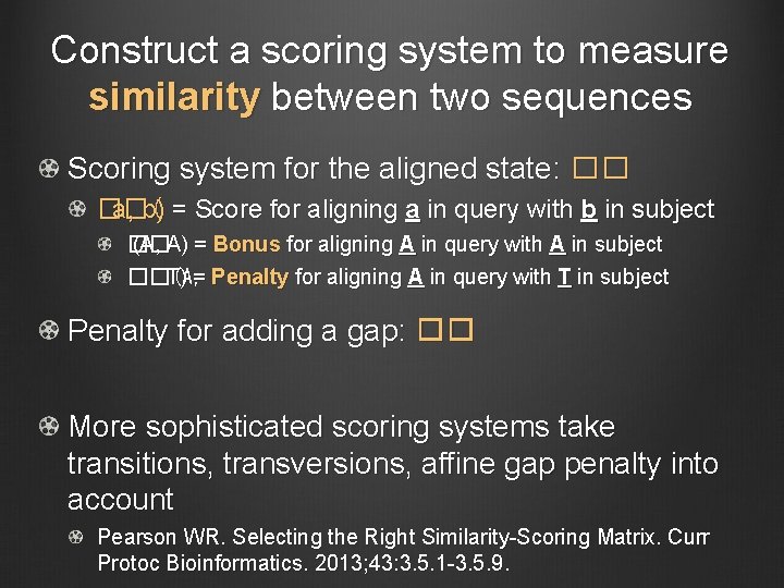
Construct a scoring system to measure similarity between two sequences Scoring system for the aligned state: �� ��( a, b) = Score for aligning a in query with b in subject �� (A, A) = Bonus for aligning A in query with A in subject ��(A, T) = Penalty for aligning A in query with T in subject Penalty for adding a gap: �� More sophisticated scoring systems take transitions, transversions, affine gap penalty into account Pearson WR. Selecting the Right Similarity-Scoring Matrix. Curr Protoc Bioinformatics. 2013; 43: 3. 5. 1 -3. 5. 9.

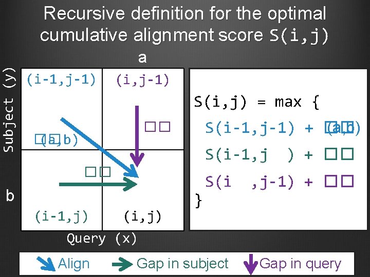
Subject (y) Recursive definition for the optimal cumulative alignment score S(i, j) a (i-1, j-1) (i, j-1) S(i, j) = max { S(i-1, j-1) + �� (a, b) �� �� (a, b) S(i-1, j �� b (i-1, j) (i, j) } S(i ) + �� , j-1) + �� Query (x) Align Gap in subject Gap in query

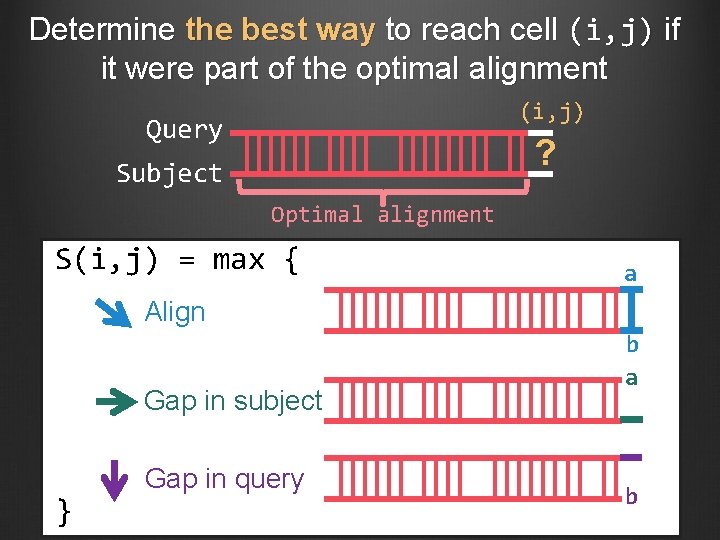
Determine the best way to reach cell (i, j) if it were part of the optimal alignment (i, j) Query ? Subject Optimal alignment S(i, j) = max { a Align Gap in subject } Gap in query b a b

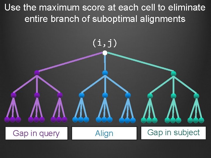
Use the maximum score at each cell to eliminate entire branch of suboptimal alignments (i, j) Gap in query Align Gap in subject

Cumulative score S(i, j) encapsulates the alignment decisions up to position (i, j) All potential optimal alignments that go through cell (i, j) have the same ancestry Re-use the cumulative alignment score (memoization) Gaps are described by the cumulative score Do not affect the coordinates of the alignment matrix Do not know the optimal alignment until we complete the entire alignment matrix Optimal alignment has the highest cumulative score

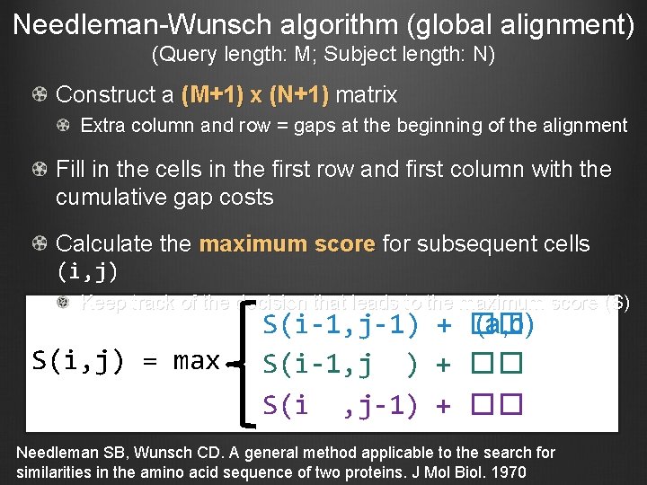
Needleman-Wunsch algorithm (global alignment) (Query length: M; Subject length: N) Construct a (M+1) x (N+1) matrix Extra column and row = gaps at the beginning of the alignment Fill in the cells in the first row and first column with the cumulative gap costs Calculate the maximum score for subsequent cells (i, j) Keep track of the decision that leads to the maximum score (S) S(i, j) = max S(i-1, j-1) + �� (a, b) S(i-1, j ) + �� S(i , j-1) + �� Needleman SB, Wunsch CD. A general method applicable to the search for similarities in the amino acid sequence of two proteins. J Mol Biol. 1970

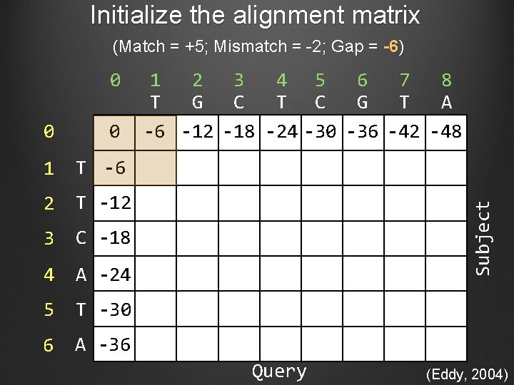
Initialize the alignment matrix (Match = +5; Mismatch = -2; Gap = -6) 0 0 1 T -6 2 T -12 3 C -18 4 A -24 5 T -30 6 A -36 1 2 3 4 5 6 7 8 T G C T C G T A -6 -12 -18 -24 -30 -36 -42 -48 Subject 0 Query (Eddy, 2004)

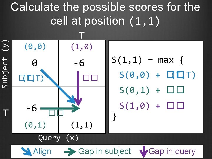
Subject (y) Calculate the possible scores for the cell at position (1, 1) T T (0, 0) (1, 0) 0 -6 �� (T, T) S(1, 1) = max { S(0, 0) + �� (T, T) �� S(0, 1) + �� -6 �� (0, 1) (1, 1) } S(1, 0) + �� Query (x) Align Gap in subject Gap in query

Subject (y) Calculate the optimal score for the cell at position (1, 1) T T S(1, 1) = max { 0 -6 -6 -6 + (-6) = -12 5 -12 -6 + (-6) = -12 5 +5 -6 -6 0 + (+5) = 5 } S(1, 1) = 5 Query (x) (Match = +5; Mismatch = -2; Gap = -6)

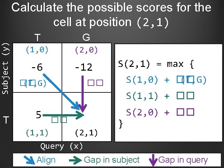
Subject (y) Calculate the possible scores for the cell at position (2, 1) T T G (1, 0) (2, 0) -6 -12 �� (T, G) S(2, 1) = max { S(1, 0) + �� (T, G) �� S(1, 1) + �� 5 �� (1, 1) (2, 1) } S(2, 0) + �� Query (x) Align Gap in subject Gap in query

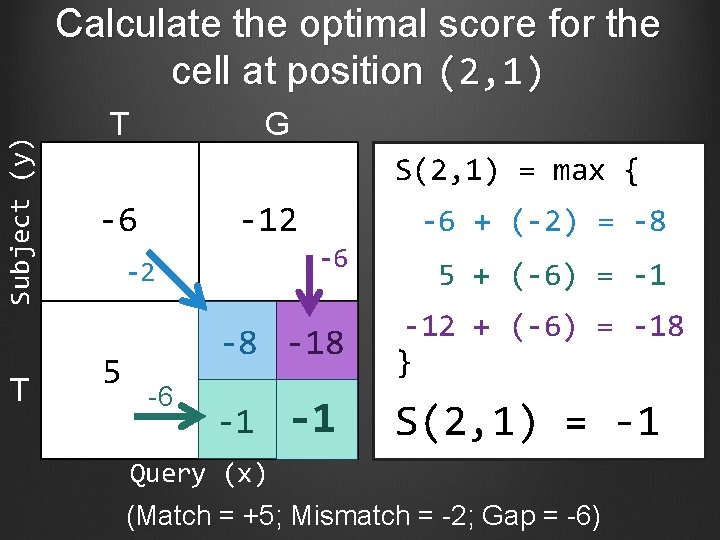
Subject (y) Calculate the optimal score for the cell at position (2, 1) T T G S(2, 1) = max { -6 -12 -6 -2 5 -6 + (-2) = -8 -8 -18 -6 -1 -1 5 + (-6) = -1 -12 + (-6) = -18 } S(2, 1) = -1 Query (x) (Match = +5; Mismatch = -2; Gap = -6)

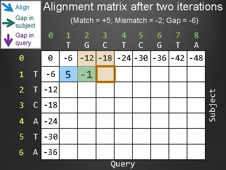
Alignment matrix after two iterations Gap in subject Gap in query (Match = +5; Mismatch = -2; Gap = -6) 0 0 0 1 T -6 2 T -12 3 C -18 4 A -24 5 T -30 6 A -36 1 2 3 4 5 6 7 8 T G C T C G T A -6 -12 -18 -24 -30 -36 -42 -48 5 -1 Subject Align Query

Subject (y) Calculate the optimal score for the cell at position (3, 1) T G C S(3, 1) = max { -12 -18 -6 -2 -1 -12 + (-2) = -14 -24 -6 -7 -7 -1 + (-6) = -7 -18 + (-6) = -24 } S(3, 1) = -7 Query (x) (Match = +5; Mismatch = -2; Gap = -6)

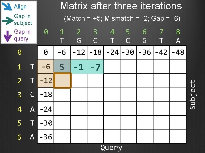
Matrix after three iterations Align Gap in subject 0 0 0 1 T -6 2 T -12 3 C -18 4 A -24 5 T -30 6 A -36 1 2 3 4 5 6 7 8 T G C T C G T A -6 -12 -18 -24 -30 -36 -42 -48 5 -1 -7 Subject Gap in query (Match = +5; Mismatch = -2; Gap = -6) Query

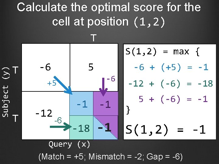
Calculate the optimal score for the cell at position (1, 2) T Subject (y) S(1, 2) = max { T -6 5 -6 +5 T -12 -6 -6 + (+5) = -1 -12 + (-6) = -18 5 + (-6) = -1 -1 -1 } -18 -1 S(1, 2) = -1 Query (x) (Match = +5; Mismatch = -2; Gap = -6)

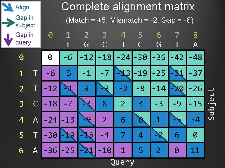
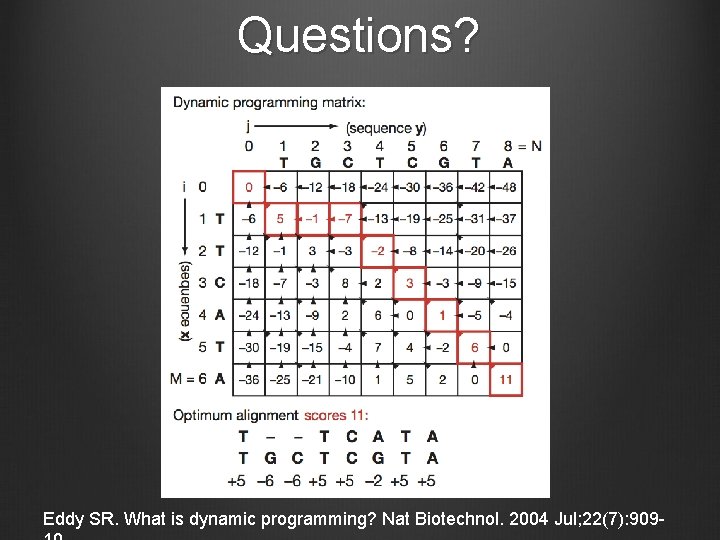
Complete alignment matrix Align Gap in subject 0 1 2 3 4 5 6 7 8 T G C T C G T A -6 -12 -18 -24 -30 -36 -42 -48 0 0 1 T -6 2 T -12 -1 3 -3 -2 -8 -14 -20 -26 3 C -18 -7 -3 8 2 3 -3 -9 -15 4 A -24 -13 -9 2 6 0 1 -5 -4 5 T -30 -19 -15 -4 7 4 -2 6 0 6 A -36 -25 -21 -10 1 5 Query 2 0 11 5 -1 -7 -13 -19 -25 -31 -37 Subject Gap in query (Match = +5; Mismatch = -2; Gap = -6)

Use traceback to recover the optimal alignment Start from the cell within the last row and last column that has the highest score Recall the step (color) that leads to this optimal score Report this step in the alignment output All the alignment decisions have already been made Repeat until we reached the beginning of the sequence Two options if multiple paths produce the same

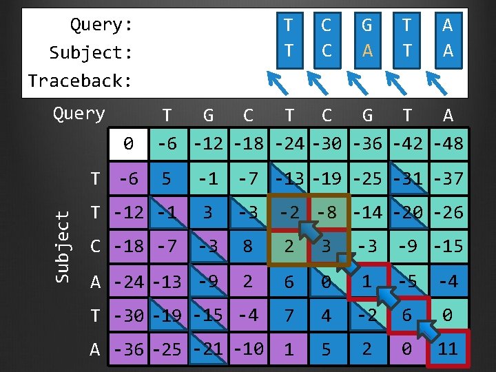
Query: Subject: Traceback: Query 0 Subject T -6 T T C C G A T T A A T G C T C G T A -6 -12 -18 -24 -30 -36 -42 -48 5 -1 -7 -13 -19 -25 -31 -37 T -12 -1 3 -3 -2 -8 -14 -20 -26 C -18 -7 -3 8 2 3 -3 -9 -15 A -24 -13 -9 2 6 0 1 -5 -4 T -30 -19 -15 -4 7 4 -2 6 0 A -36 -25 -21 -10 1 5 2 0 11

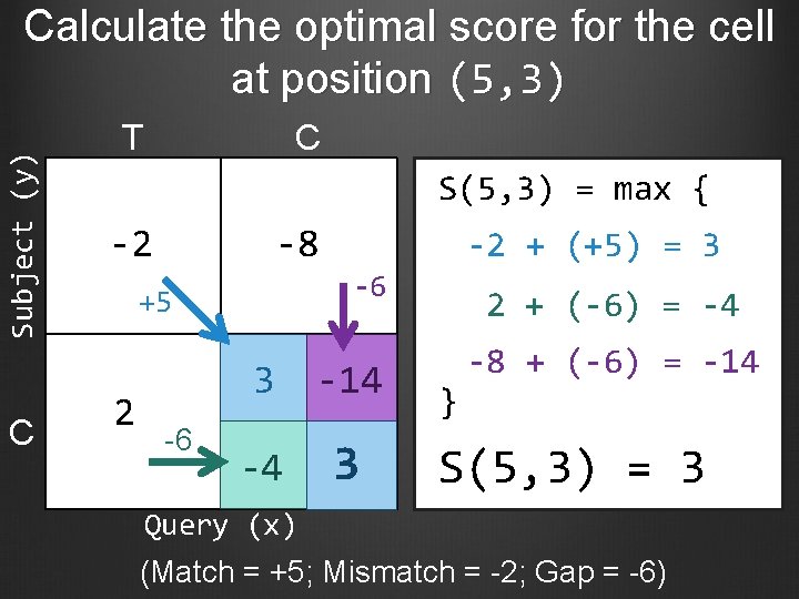
Subject (y) Calculate the optimal score for the cell at position (5, 3) C T C S(5, 3) = max { -2 -8 -6 +5 2 -6 -2 + (+5) = 3 3 -14 -4 3 2 + (-6) = -4 } -8 + (-6) = -14 S(5, 3) = 3 Query (x) (Match = +5; Mismatch = -2; Gap = -6)

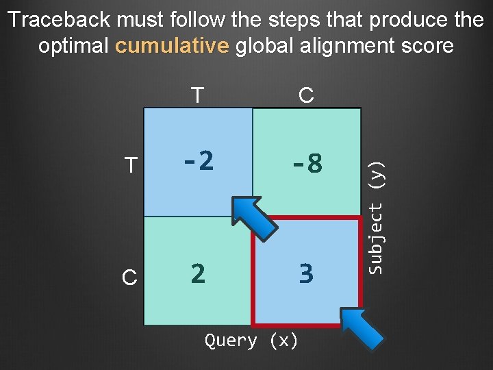
T C T -2 -8 C 2 3 Query (x) Subject (y) Traceback must follow the steps that produce the optimal cumulative global alignment score

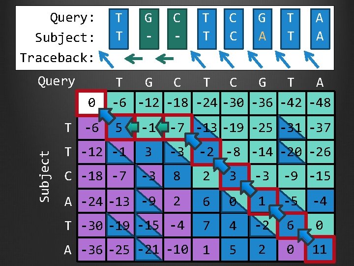
Query: Subject: Traceback: Query 0 Subject T -6 T T G - C - T T C C G A T T A A T G C T C G T A -6 -12 -18 -24 -30 -36 -42 -48 5 -1 -7 -13 -19 -25 -31 -37 T -12 -1 3 -3 -2 -8 -14 -20 -26 C -18 -7 -3 8 2 3 -3 -9 -15 A -24 -13 -9 2 6 0 1 -5 -4 T -30 -19 -15 -4 7 4 -2 6 0 A -36 -25 -21 -10 1 5 2 0 11

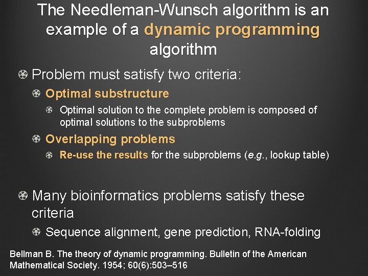
The Needleman-Wunsch algorithm is an example of a dynamic programming algorithm Problem must satisfy two criteria: Optimal substructure Optimal solution to the complete problem is composed of optimal solutions to the subproblems Overlapping problems Re-use the results for the subproblems (e. g. , lookup table) Many bioinformatics problems satisfy these criteria Sequence alignment, gene prediction, RNA-folding Bellman B. The theory of dynamic programming. Bulletin of the American Mathematical Society. 1954; 60(6): 503– 516

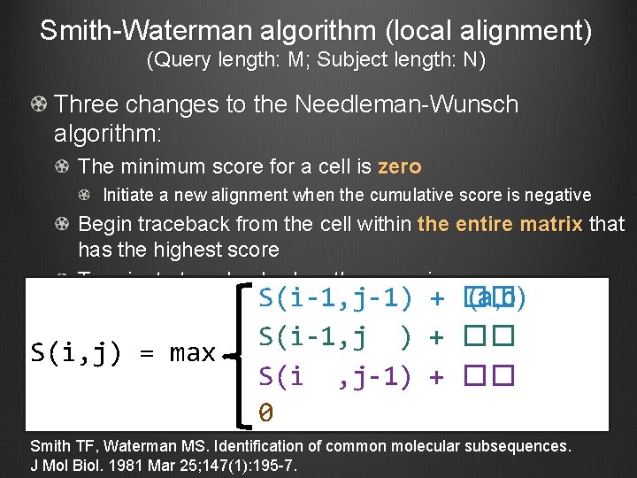
Smith-Waterman algorithm (local alignment) (Query length: M; Subject length: N) Three changes to the Needleman-Wunsch algorithm: The minimum score for a cell is zero Initiate a new alignment when the cumulative score is negative Begin traceback from the cell within the entire matrix that has the highest score Terminate traceback when the score is zero S(i, j) = max S(i-1, j-1) + �� (a, b) S(i-1, j ) + �� S(i , j-1) + �� 0 Smith TF, Waterman MS. Identification of common molecular subsequences. J Mol Biol. 1981 Mar 25; 147(1): 195 -7.

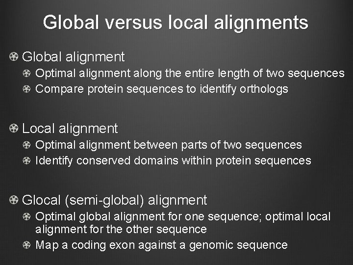
Global versus local alignments Global alignment Optimal alignment along the entire length of two sequences Compare protein sequences to identify orthologs Local alignment Optimal alignment between parts of two sequences Identify conserved domains within protein sequences Glocal (semi-global) alignment Optimal global alignment for one sequence; optimal local alignment for the other sequence Map a coding exon against a genomic sequence

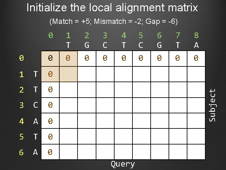
Initialize the local alignment matrix (Match = +5; Mismatch = -2; Gap = -6) 0 0 1 T 0 2 T 0 3 C 0 4 A 0 5 T 0 6 A 0 1 T 0 2 G 0 3 C 0 4 T 0 5 C 0 6 G 0 7 T 0 8 A 0 Subject 0 Query

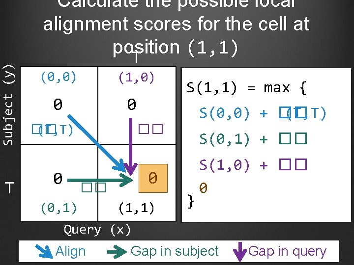
Subject (y) T Calculate the possible local alignment scores for the cell at position (1, 1) T (0, 0) (1, 0) 0 0 �� (T, T) 0 S(1, 1) = max { S(0, 0) + �� (T, T) �� 0 �� (0, 1) S(0, 1) + �� (1, 1) } S(1, 0) + �� 0 Query (x) Align Gap in subject Gap in query

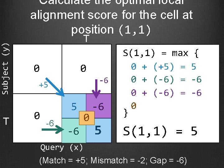
Subject (y) Calculate the optimal local alignment score for the cell at position (1, 1) T T 0 0 -6 +5 0 5 -6 0 -6 -6 5 S(1, 1) = max { 0 + (+5) = 5 0 + (-6) = -6 0 } S(1, 1) = 5 Query (x) (Match = +5; Mismatch = -2; Gap = -6)

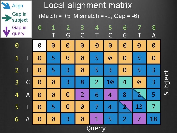
Gap in subject (Match = +5; Mismatch = -2; Gap = -6) Gap in query 0 0 0 1 T 0 2 G 0 3 C 0 4 T 0 5 C 0 6 G 0 7 T 0 8 A 0 1 T 0 5 0 2 T 0 5 3 3 C 0 0 3 8 2 10 4 0 3 4 A 0 0 0 2 6 4 8 2 5 5 T 0 5 0 0 7 4 2 13 7 6 A 0 0 3 0 1 5 Query 2 7 18 Subject Local alignment matrix Align

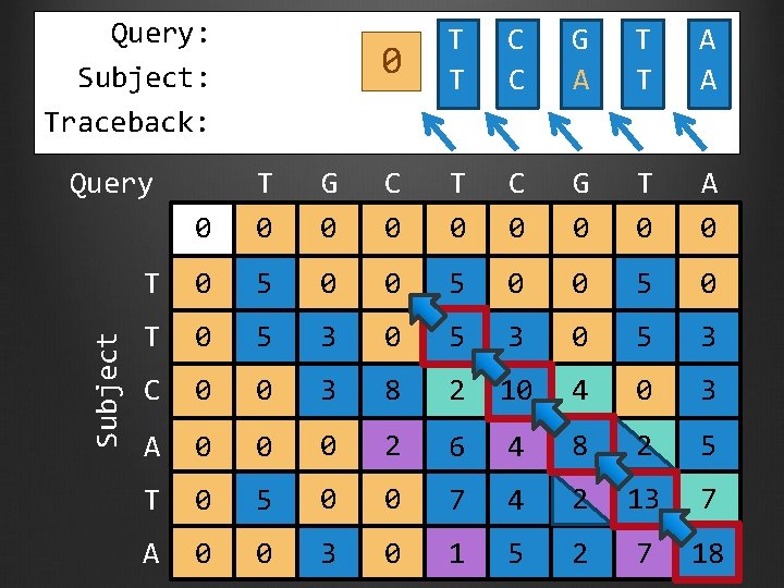
Query: Subject: Traceback: Subject Query 0 T T C C G A T T A A 0 T 0 G 0 C 0 T 0 C 0 G 0 T 0 A 0 T 0 5 0 T 0 5 3 C 0 0 3 8 2 10 4 0 3 A 0 0 0 2 6 4 8 2 5 T 0 5 0 0 7 4 2 13 7 A 0 0 3 0 1 5 2 7 18

Techniques to improve the performance of sequence alignment Time and space complexity: O(MN) Double the size of the two sequences leads to a fourfold increase in the amount of time and space required Reduce memory requirement Myers EW, Miller W. Optimal alignments in linear space. Comput Appl Biosci. 1988 Mar; 4(1): 11 -7. Fill the matrix in parallel (SIMD, CUDA) Farrar M. Striped Smith-Waterman speeds database searches six times over other SIMD implementations. Bioinformatics. 2007 Jan 15; 23(2): 15661. Find high-scoring instead of the best alignment Altschul SF, Gish W, Miller W, Myers EW, Lipman DJ. Basic local alignment search tool. J Mol Biol. 1990 Oct 5; 215(3): 403 -10.

Questions? Eddy SR. What is dynamic programming? Nat Biotechnol. 2004 Jul; 22(7): 909 -

Rationale for calculating the scores for the entire alignment matrix Cannot determine the best global alignment without aligning the entire query and subject sequences Cannot evaluate all possible alignments If the alignment before we reached cell (i, j) is part of the optimal alignment: Identify the next step (i. e. align, gap in query, gap in subject) that will be part of the optimal alignment Use traceback to determine the final alignment Different alignments could produce the same score

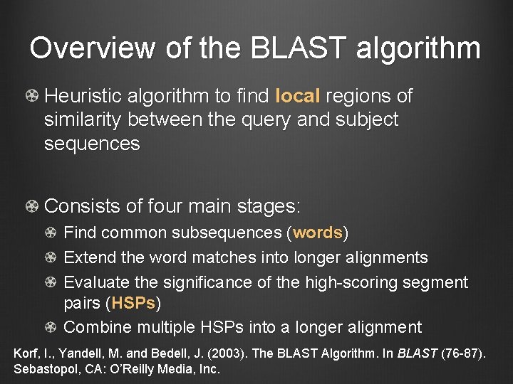
Overview of the BLAST algorithm Heuristic algorithm to find local regions of similarity between the query and subject sequences Consists of four main stages: Find common subsequences (words) Extend the word matches into longer alignments Evaluate the significance of the high-scoring segment pairs (HSPs) Combine multiple HSPs into a longer alignment Korf, I. , Yandell, M. and Bedell, J. (2003). The BLAST Algorithm. In BLAST (76 -87). Sebastopol, CA: O’Reilly Media, Inc.

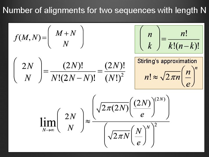
Number of alignments for two sequences with length N Stirling’s approximation

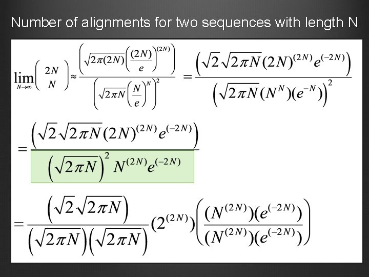
Number of alignments for two sequences with length N

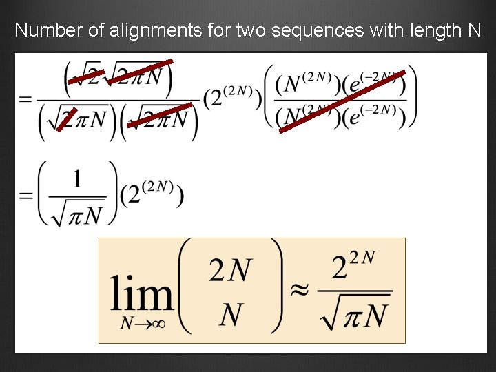
Number of alignments for two sequences with length N

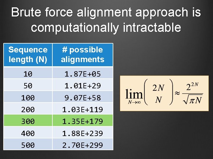
Brute force alignment approach is computationally intractable Sequence length (N) # possible alignments 10 50 100 200 300 400 500 1. 87 E+05 1. 01 E+29 9. 07 E+58 1. 03 E+119 1. 35 E+179 1. 88 E+239 2. 70 E+299