Introduction to Digital Signal Processing DSP Part 2

Introduction to Digital Signal Processing (DSP) Part 2 of 4 (“Power Spectral Density Basics”) James R. (Jim) Beaty, Ph. D - NASA Langley Research Center Vehicle Analysis Branch, Systems Analysis & Concepts Directorate Bldg 1209, Room 128 B, M/S 451 1 North Dryden Street Hampton, VA 23681 757 -864 -1322 James. R. Beaty@nasa. gov Learning from the Past, Looking to the Future Page: 1

Overview • Part 1, “Mathematical Concepts” – Definitions, mathematical pre-requisites, and application techniques • Fourier transforms and convolution • Discrete Fourier transforms (DFT) and Fast Fourier transforms (FFT) • Shannon Sampling Theorem and data aliasing • Part 2, “Power Spectral Density Basics” – Power Spectral Density (PSD) to estimate spectral characteristics of waveforms – PSD Demonstration • Part 3 “Implementing Discrete Filters” – Converting from continuous Laplace domain filters to discrete Z-domain filters (Tustin’s rule, or bilinear transformation) – Recursive filter implementations for discrete filters • Part 4 “Typical GN&C Applications” – – – Normalized frequency Methods to verify transfer function magnitude/phase of discrete filters using DFT (or FFT) Example use of discrete filter to implement a notch filter Learning from the Past, Looking to the Future Page: 2

Power Spectral Density (PSD) • Power spectral density, or PSD, is a technique for estimating the spectral (i. e. – frequency) content of signal waveforms • PSDs use FFTs to compute the discrete Fourier transforms (DFTs) of the input signal to extract its frequency content • PSD is useful for evaluating periodic content of signals from some device (e. g. – sensors) to characterize for modeling or requirements compliance • PSD represents the density of the signal squared magnitude at a particular frequency, e. g. – units^2 per hertz – The integral of a signal’s PSD provides the signal’s mean square value – Nonzero mean signals are usually “detrended” (e. g. – remove the mean value) before computing the PSD Learning from the Past, Looking to the Future Page: 3

DFT size and sampling • • Before continuing with the PSD discussion, provide a few comments about characteristics of DFT size, sampling, and windowing on the calculation of the DFT used in PSD analysis The DFT size used in computing PSDs affects the resolution of the calculation of the spectral content of the data – Larger DFT sizes increase the resolution of the calculations – Higher resolution can introduce some unexpected results (more to follow on this) The placement of spectral content in the sampled data with respect to the DFT “basis frequencies” can affect the output DFT calculation (more to follow on this) The use of “windows” in the calculation of the DFT can eliminate some of these issues that will be discussed Learning from the Past, Looking to the Future Page: 4

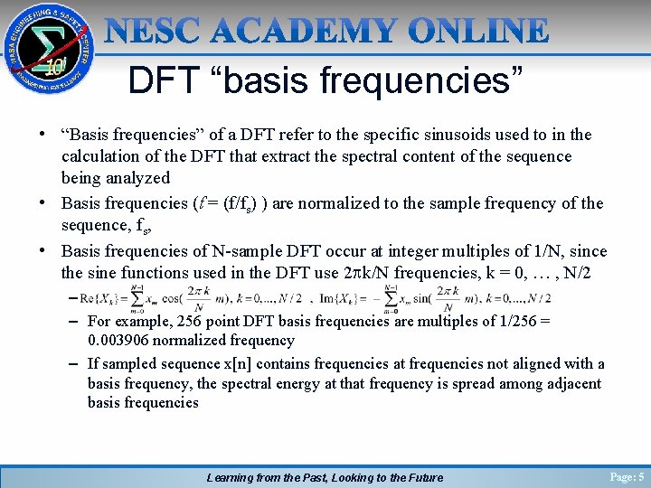
DFT “basis frequencies” • “Basis frequencies” of a DFT refer to the specific sinusoids used to in the calculation of the DFT that extract the spectral content of the sequence being analyzed • Basis frequencies (ƭ = (f/fs) ) are normalized to the sample frequency of the sequence, fs, • Basis frequencies of N-sample DFT occur at integer multiples of 1/N, since the sine functions used in the DFT use 2 pk/N frequencies, k = 0, … , N/2 – – For example, 256 point DFT basis frequencies are multiples of 1/256 = 0. 003906 normalized frequency – If sampled sequence x[n] contains frequencies at frequencies not aligned with a basis frequency, the spectral energy at that frequency is spread among adjacent basis frequencies Learning from the Past, Looking to the Future Page: 5

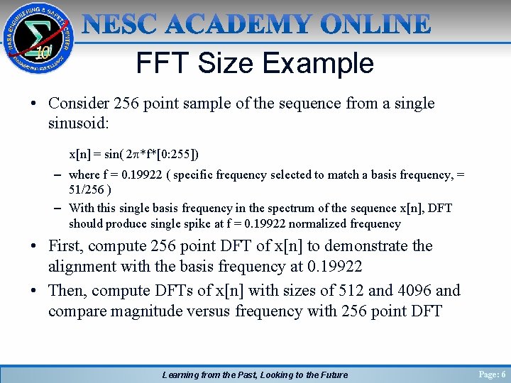
FFT Size Example • Consider 256 point sample of the sequence from a single sinusoid: x[n] = sin( 2 p*f*[0: 255]) – where f = 0. 19922 ( specific frequency selected to match a basis frequency, = 51/256 ) – With this single basis frequency in the spectrum of the sequence x[n], DFT should produce single spike at f = 0. 19922 normalized frequency • First, compute 256 point DFT of x[n] to demonstrate the alignment with the basis frequency at 0. 19922 • Then, compute DFTs of x[n] with sizes of 512 and 4096 and compare magnitude versus frequency with 256 point DFT Learning from the Past, Looking to the Future Page: 6

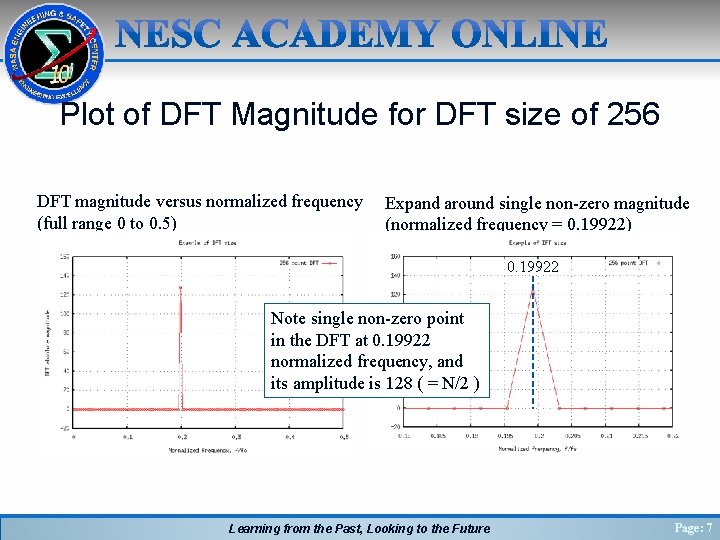
Plot of DFT Magnitude for DFT size of 256 DFT magnitude versus normalized frequency Expand around single non-zero magnitude (full range 0 to 0. 5) (normalized frequency = 0. 19922) 0. 19922 Note single non-zero point in the DFT at 0. 19922 normalized frequency, and its amplitude is 128 ( = N/2 ) Learning from the Past, Looking to the Future Page: 7

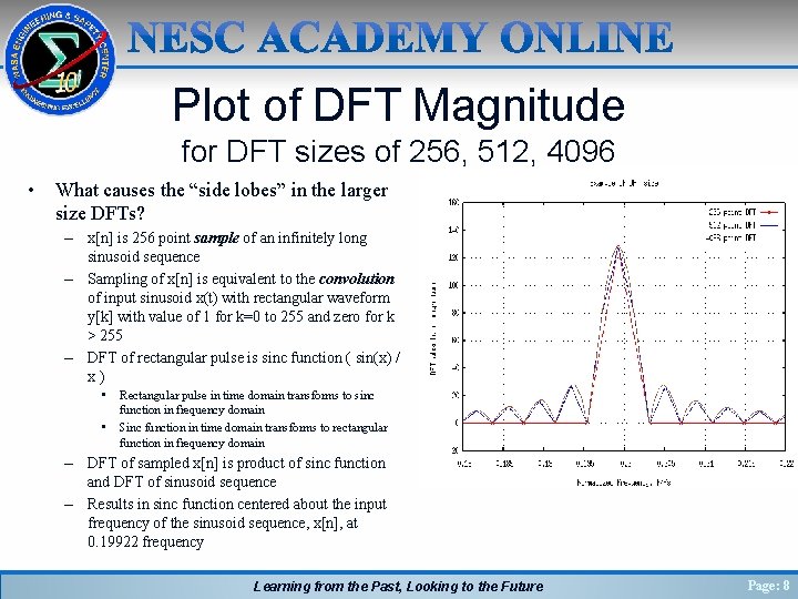
Plot of DFT Magnitude for DFT sizes of 256, 512, 4096 • What causes the “side lobes” in the larger size DFTs? – x[n] is 256 point sample of an infinitely long sinusoid sequence – Sampling of x[n] is equivalent to the convolution of input sinusoid x(t) with rectangular waveform y[k] with value of 1 for k=0 to 255 and zero for k > 255 – DFT of rectangular pulse is sinc function ( sin(x) / x ) • • Rectangular pulse in time domain transforms to sinc function in frequency domain Sinc function in time domain transforms to rectangular function in frequency domain – DFT of sampled x[n] is product of sinc function and DFT of sinusoid sequence – Results in sinc function centered about the input frequency of the sinusoid sequence, x[n], at 0. 19922 frequency Learning from the Past, Looking to the Future Page: 8

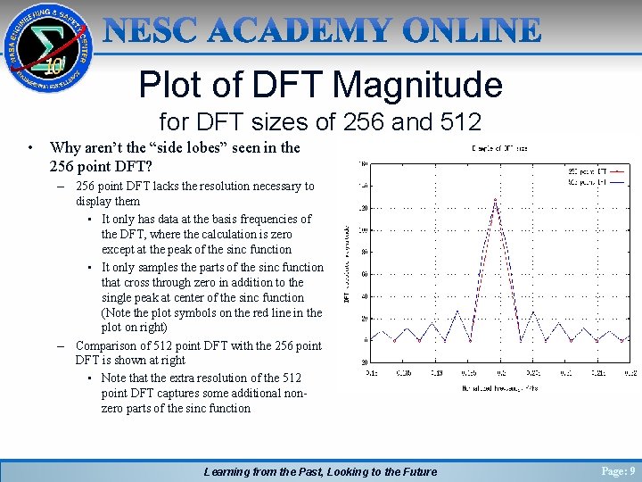
Plot of DFT Magnitude for DFT sizes of 256 and 512 • Why aren’t the “side lobes” seen in the 256 point DFT? – 256 point DFT lacks the resolution necessary to display them • It only has data at the basis frequencies of the DFT, where the calculation is zero except at the peak of the sinc function • It only samples the parts of the sinc function that cross through zero in addition to the single peak at center of the sinc function (Note the plot symbols on the red line in the plot on right) – Comparison of 512 point DFT with the 256 point DFT is shown at right • Note that the extra resolution of the 512 point DFT captures some additional nonzero parts of the sinc function Learning from the Past, Looking to the Future Page: 9

DFT and “basis frequencies” • In the example just presented, the 0. 19922 normalized frequency of the input sinusoid sequence, x[n], was carefully chosen to align exactly with one of the basis frequencies of the DFT which occur at integer multiples of 1/256 for a 256 point DFT • What happens if the input sequence is not so carefully contrived? • For this second example, change the normalized frequency of the input sequence from 0. 19922 to 0. 2, again using 256 point samples and a 256 point DFT That is: x[n] = sin( 2 p*0. 2 * [0: 255] ) , n = 0 , … , 255 Learning from the Past, Looking to the Future Page: 10

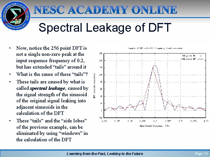
Spectral Leakage of DFT • • Now, notice the 256 point DFT is not a single non-zero peak at the input sequence frequency of 0. 2, but has extended “tails” around it What is the cause of these “tails”? These tails are caused by what is called spectral leakage, caused by the signal strength of the sinusoid of the original signal leaking into adjacent sinusoids in the calculation of the DFT These “tails” and the “side lobes” of the previous example, can be eliminated by using “windows” in the calculation of the DFT Learning from the Past, Looking to the Future Page: 11

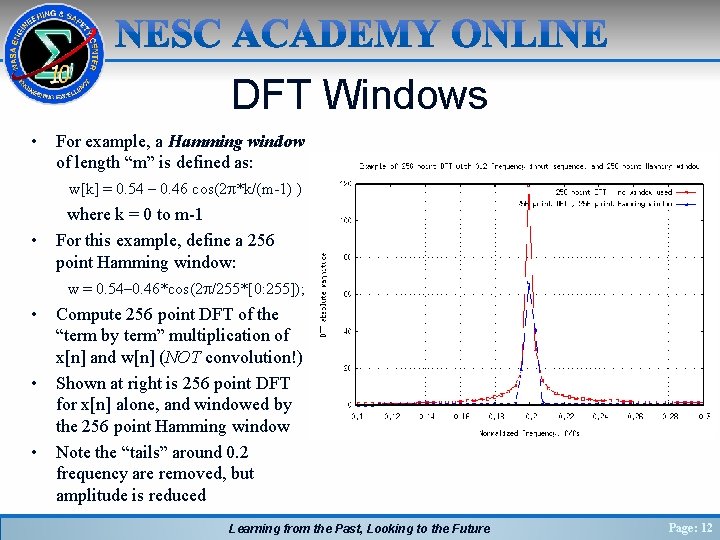
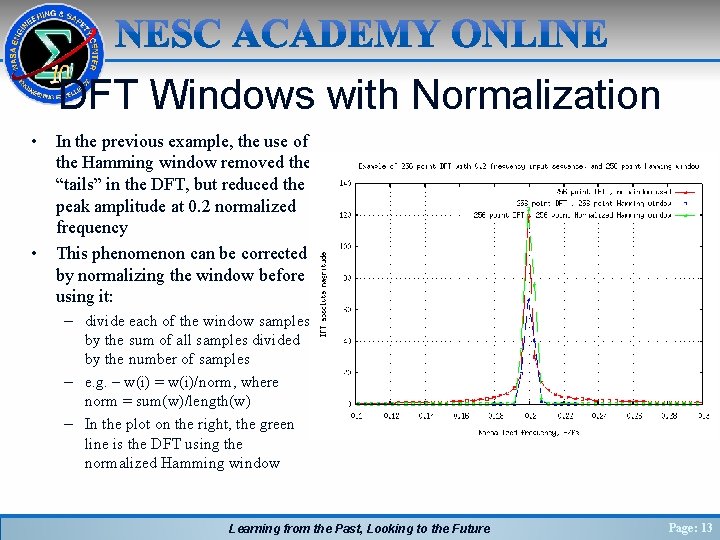
DFT Windows • For example, a Hamming window of length “m” is defined as: w[k] = 0. 54 – 0. 46 cos(2 p*k/(m-1) ) where k = 0 to m-1 • For this example, define a 256 point Hamming window: w = 0. 54– 0. 46*cos(2 p/255*[0: 255]); • • • Compute 256 point DFT of the “term by term” multiplication of x[n] and w[n] (NOT convolution!) Shown at right is 256 point DFT for x[n] alone, and windowed by the 256 point Hamming window Note the “tails” around 0. 2 frequency are removed, but amplitude is reduced Learning from the Past, Looking to the Future Page: 12

DFT Windows with Normalization • • In the previous example, the use of the Hamming window removed the “tails” in the DFT, but reduced the peak amplitude at 0. 2 normalized frequency This phenomenon can be corrected by normalizing the window before using it: – divide each of the window samples by the sum of all samples divided by the number of samples – e. g. – w(i) = w(i)/norm, where norm = sum(w)/length(w) – In the plot on the right, the green line is the DFT using the normalized Hamming window Learning from the Past, Looking to the Future Page: 13

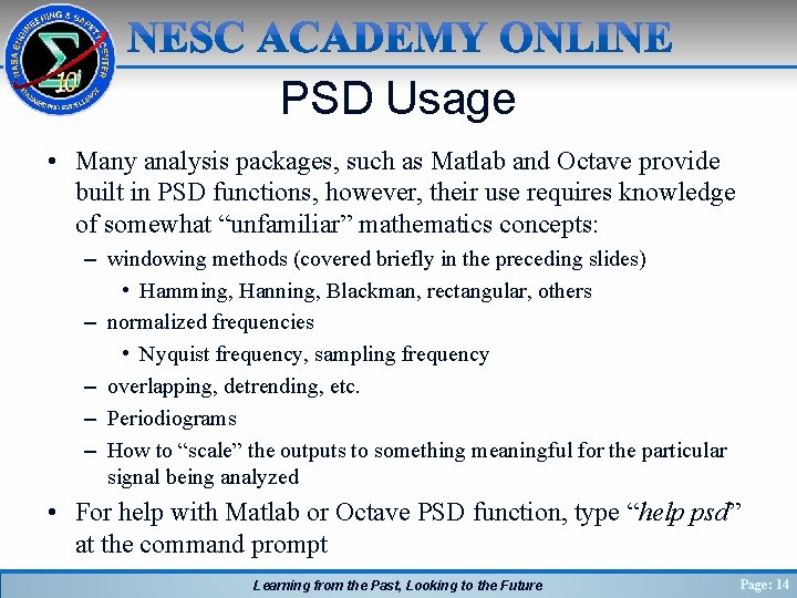
PSD Usage • Many analysis packages, such as Matlab and Octave provide built in PSD functions, however, their use requires knowledge of somewhat “unfamiliar” mathematics concepts: – windowing methods (covered briefly in the preceding slides) • Hamming, Hanning, Blackman, rectangular, others – normalized frequencies • Nyquist frequency, sampling frequency – overlapping, detrending, etc. – Periodiograms – How to “scale” the outputs to something meaningful for the particular signal being analyzed • For help with Matlab or Octave PSD function, type “help psd” at the command prompt Learning from the Past, Looking to the Future Page: 14

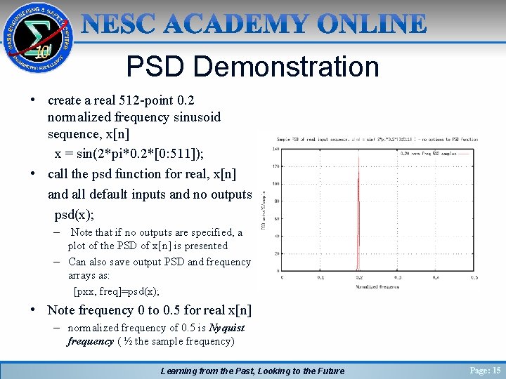
PSD Demonstration • create a real 512 -point 0. 2 normalized frequency sinusoid sequence, x[n] x = sin(2*pi*0. 2*[0: 511]); • call the psd function for real, x[n] and all default inputs and no outputs psd(x); – Note that if no outputs are specified, a plot of the PSD of x[n] is presented – Can also save output PSD and frequency arrays as: [pxx, freq]=psd(x); • Note frequency 0 to 0. 5 for real x[n] – normalized frequency of 0. 5 is Nyquist frequency ( ½ the sample frequency) Learning from the Past, Looking to the Future Page: 15

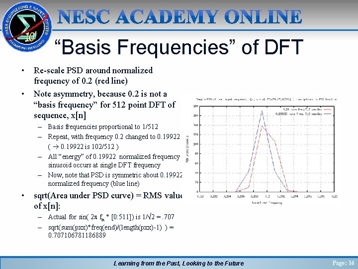
“Basis Frequencies” of DFT • • Re-scale PSD around normalized frequency of 0. 2 (red line) Note asymmetry, because 0. 2 is not a “basis frequency” for 512 point DFT of sequence, x[n] – Basis frequencies proportional to 1/512 – Repeat, with frequency 0. 2 changed to 0. 19922 ( 0. 19922 is 102/512 ) – All “energy” of 0. 19922 normalized frequency sinusoid occurs at single DFT frequency – Now, note that PSD is symmetric about 0. 19922 normalized frequency (blue line) • sqrt(Area under PSD curve) = RMS value of x[n]: – Actual for sin( 2 p fn * [0: 511]) is 1/√ 2 =. 707 – sqrt(sum(pxx)*freq(end)/(length(pxx)-1) ) = 0. 707106781186889 Learning from the Past, Looking to the Future Page: 16

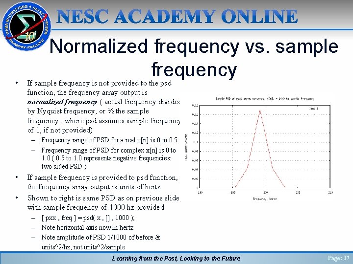
• Normalized frequency vs. sample frequency If sample frequency is not provided to the psd function, the frequency array output is normalized frequency ( actual frequency divided by Nyquist frequency, or ½ the sample frequency , where psd assumes sample frequency of 1, if not provided) – Frequency range of PSD for a real x[n] is 0 to 0. 5 – Frequency range of PSD for complex x[n] is 0 to 1. 0 ( 0. 5 to 1. 0 represents negative frequencies: two sided PSD ) • • If sample frequency is provided to psd function, the frequency array output is units of hertz Shown to right is same PSD as on previous slide, with sample frequency of 1000 hz provided – [ pxx , freq ] = psd( x , [] , 1000 ); – Note horizontal axis now in hertz – Note amplitude of PSD 1/1000 of before & units^2/hz, not units^2/sample Learning from the Past, Looking to the Future Page: 17

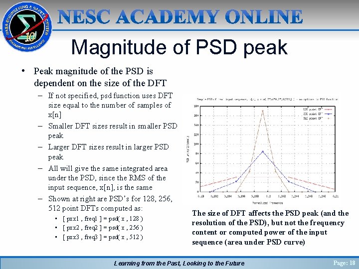
Magnitude of PSD peak • Peak magnitude of the PSD is dependent on the size of the DFT – If not specified, psd function uses DFT size equal to the number of samples of x[n] – Smaller DFT sizes result in smaller PSD peak – Larger DFT sizes result in larger PSD peak – All will give the same integrated area under the PSD, since the RMS of the input sequence, x[n], is the same – Shown at right are PSD’s for 128, 256, 512 point DFTs computed as: • [ pxx 1 , freq 1 ] = psd( x , 128 ) • [ pxx 2 , freq 2 ] = psd( x , 256 ) • [ pxx 3 , freq 3 ] = psd( x , 512 ) The size of DFT affects the PSD peak (and the resolution of the PSD), but not the frequency content or computed power of the input sequence (area under PSD curve) Learning from the Past, Looking to the Future Page: 18

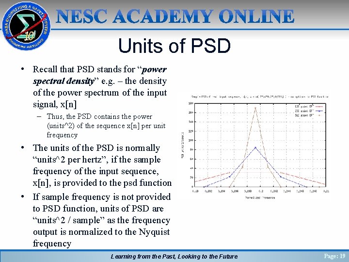
Units of PSD • Recall that PSD stands for “power spectral density” e. g. – the density of the power spectrum of the input signal, x[n] – Thus, the PSD contains the power (units^2) of the sequence x[n] per unit frequency • The units of the PSD is normally “units^2 per hertz”, if the sample frequency of the input sequence, x[n], is provided to the psd function • If sample frequency is not provided to PSD function, units of PSD are “units^2 / sample” as the frequency output is normalized to the Nyquist frequency Learning from the Past, Looking to the Future Page: 19

Complex sequence • • (two sided PSD) Create a complex sequence, xc[n], by adding 0. 00001*i to one of the elements of the previous real sequence x[n]: xc = x; xc(1) = xc(1) + 0. 00001*i; call the psd function all default inputs and outputs, pxx and freq: [pxx, freq] = psd(xc); Plot the PSD of the complex sequence, xc[n] in blue along with the PSD of the real sequence, x[n] in red Note that the frequency range is now 0. 0 to 1. 0. – – The negative frequencies are 0. 5 to 1. 0 • 0. 8 normalized frequency is same as -0. 2 Also note that the amplitude of the PSD is half that of the PSD of the real sequence, x[n] (e. g. – twosided PSD compared with one-sided PSD) 0 to +0. 5 Learning from the Past, Looking to the Future +0. 5 & -0. 5 0 to -0. 5 Page: 20

PSD Window Options • Compute 4096 point PSD of real sequence, x[n] with frequency of 199. 22 hz and illustrate different window options available: – – – negative window size , n = n-point rectangular window (average the n-point PSDs) [pxx 1, freq 1] = psd( x, 4096, 1000, -128) 128 point Hanning window (average 128 point PSDs) – note positive integer window input, defaults to hanning window of that length [pxx 2, freq 2] = psd( x, 4096, 1000, 128); 128 point Hanning window (average 128 point PSDs) – note string window input [pxx 3, freq 3] = psd( x, 4096, 1000, ’hanning(128)’); 128 point Hamming window (average 128 point PSDs) – note string window input [pxx 4, freq 4] = psd( x, 4096, 1000, ’hamming(128)’); 128 point Blackman window string input – average the 128 point PSDs [pxx 5, freq 5] = psd( x, 4096, 1000, 'blackman(128)' ); Frequency, hz Learning from the Past, Looking to the Future Page: 21

PSD as “Averaged Periodograms” • When windows are used that are smaller size than the length of the sequence, x[n] being analyzed, the PSDs are formed by averaging the individual PSDs computed from the smaller, windowed samples of the sequence • These averaged PSDs are called “averaged periodograms” Learning from the Past, Looking to the Future Page: 22

PSD “Detrending” & “Overlap” • “Detrending” in the calculation of a PSD refers to removing trends from the sampled data, x[n] – Trends include: • Non-zero mean value, or constant bias • Linear bias – The Matlab and Octave psd function includes a string input, “dflag” that specifies the type of detrending desired: • ‘none’ – to perform no de-trending (this is the default action) • ‘constant’ – to remove a constant bias , or mean value • ‘linear’ – to remove a linear bias • “Overlap” is similar to averaging used in windows, except that a specified number of adjacent, or overlapped, values of the input sequence, x[n] are included in the individual PSDs that are computed, then averaged Learning from the Past, Looking to the Future Page: 23

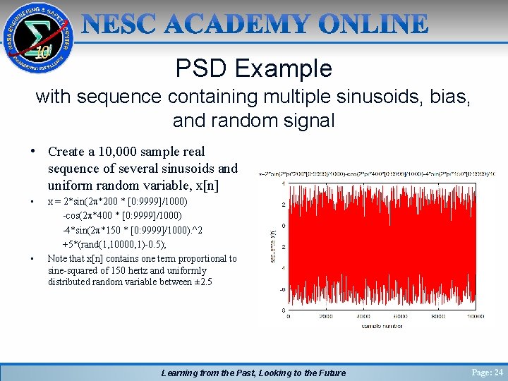
PSD Example with sequence containing multiple sinusoids, bias, and random signal • Create a 10, 000 sample real sequence of several sinusoids and uniform random variable, x[n] • • x = 2*sin(2 p*200 * [0: 9999]/1000) -cos(2 p*400 * [0: 9999]/1000) -4*sin(2 p*150 * [0: 9999]/1000). ^2 +5*(rand(1, 10000, 1)-0. 5); Note that x[n] contains one term proportional to sine-squared of 150 hertz and uniformly distributed random variable between ± 2. 5 Learning from the Past, Looking to the Future Page: 24

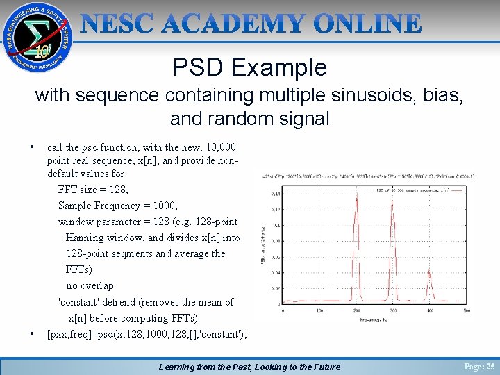
PSD Example with sequence containing multiple sinusoids, bias, and random signal • call the psd function, with the new, 10, 000 point real sequence, x[n], and provide nondefault values for: FFT size = 128, Sample Frequency = 1000, window parameter = 128 (e. g. 128 -point Hanning window, and divides x[n] into 128 -point seqments and average the FFTs) no overlap 'constant' detrend (removes the mean of x[n] before computing FFTs) • [pxx, freq]=psd(x, 128, 1000, 128, [], 'constant'); Learning from the Past, Looking to the Future Page: 25

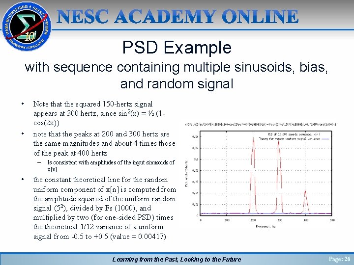
PSD Example with sequence containing multiple sinusoids, bias, and random signal • • Note that the squared 150 -hertz signal appears at 300 hertz, since sin 2(x) = ½ (1 cos(2 x)) note that the peaks at 200 and 300 hertz are the same magnitudes and about 4 times those of the peak at 400 hertz – • Is consistent with amplitudes of the input sinusoids of x[n] the constant theoretical line for the random uniform component of x[n] is computed from the amplitude squared of the uniform random signal (52), divided by Fs (1000), and multiplied by two (for one-sided PSD) times theoretical 1/12 variance of a uniform signal from -0. 5 to +0. 5 (value = 0. 00417) Learning from the Past, Looking to the Future Page: 26

PSD Example with sequence containing multiple sinusoids, bias, and random signal • • Rescale the plot to show the area around the constant theoretical line for random component of x[n] Note that the mean value of the 10, 000 point waveform, x[n], is -1. 9919, its standard deviation is 2. 5768 its RMS value is 3. 2568 Compute the RMS value of the signal, x[n], by integrating its PSD e. g. rms = sqrt( sum(pxx) * ( freq(end)/length(freq) ) rms = 2. 5669 Note that this RMS value computed from the PSD does not include the mean value of the input signal since the mean was removed by the 'detrend' PSD argument, so this “RMS” calculation should match the standard deviation of x Learning from the Past, Looking to the Future Page: 27

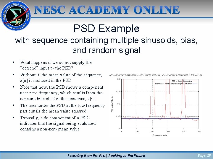
PSD Example with sequence containing multiple sinusoids, bias, and random signal • • • What happens if we do not supply the “detrend” input to the PSD? Without it, the mean value of the sequence, x[n] is included in the PSD Note that now, the PSD shows a component near zero frequency, which results from the constant bias of -2 in the sequence, x[n] The area under the PSD at the low frequency part equals the mean value squared Typically, a dc component of a PSD indicates that the signal being evaluated contains a non-zero mean value Learning from the Past, Looking to the Future Page: 28

Introduction to DSP, Part 2 of 4 Summary • In Part 1, “Mathematical Concepts” we covered the following: – Definitions, mathematical pre-requisites, and application techniques • Fourier transforms and convolution • Discrete Fourier transforms (DFT) and Fast Fourier transforms (FFT) • Shannon Sampling Theorem and data aliasing • In Part 2, “Power Spectral Density Basics”, we have covered the following: – Power Spectral Density (PSD) to estimate spectral characteristics of waveforms – PSD Demonstration • In Part 3 “Implementing Discrete Filters” we will cover the following: – Converting from continuous Laplace domain filters to discrete Z-domain filters (Tustin’s rule, or bilinear transformation) – Recursive filter implementations for discrete filters • In Part 4 “Typical GN&C Applications” we will cover the following: – – – Normalized frequency Methods to verify transfer function magnitude/phase of discrete filters using DFT (or FFT) Example use of discrete filter to implement a notch filter Learning from the Past, Looking to the Future Page: 29