Introduction to Digital Signal Processing DSP Part 1

Introduction to Digital Signal Processing (DSP) Part 1 of 4 (“Mathematical Concepts”) James R. (Jim) Beaty, Ph. D - NASA Langley Research Center Vehicle Analysis Branch, Systems Analysis & Concepts Directorate Bldg 1209, Room 128 B, M/S 451 1 North Dryden Street Hampton, VA 23681 757 -864 -1322 James. R. Beaty@nasa. gov Learning from the Past, Looking to the Future Page: 1

Overview • Part 1, “Mathematical Concepts” – Definitions, mathematical pre-requisites, and application techniques • Fourier transforms and convolution • Discrete Fourier transforms (DFT) and Fast Fourier transforms (FFT) • Shannon Sampling Theorem and data aliasing • Part 2, “Power Spectral Density Basics” – Power Spectral Density (PSD) to estimate spectral characteristics of waveforms – PSD Demonstration • Part 3 “Implementing Discrete Filters” – Converting from continuous Laplace domain filters to discrete Z-domain filters (Tustin’s rule, or bilinear transformation) – Recursive filter implementations for discrete filters • Part 4 “Typical GN&C Applications” – – – Normalized frequency Methods to verify transfer function magnitude/phase of discrete filters using DFT (or FFT) Example use of discrete filter to implement a notch filter Learning from the Past, Looking to the Future Page: 2

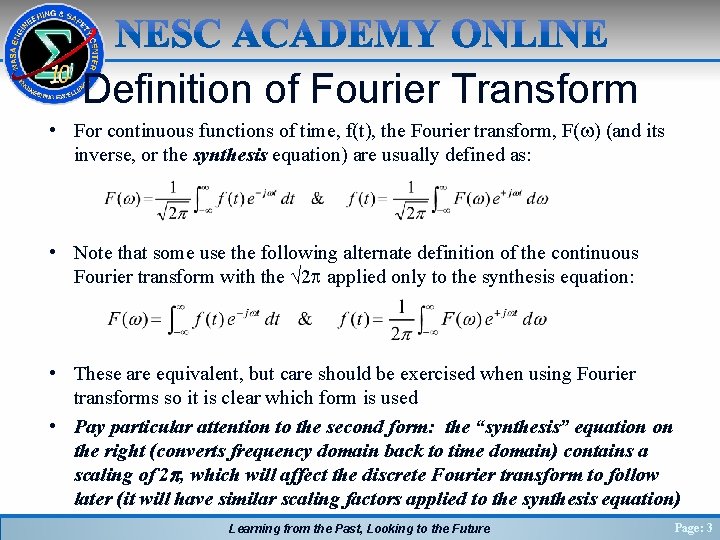
Definition of Fourier Transform • For continuous functions of time, f(t), the Fourier transform, F(w) (and its inverse, or the synthesis equation) are usually defined as: • Note that some use the following alternate definition of the continuous Fourier transform with the √ 2 p applied only to the synthesis equation: • These are equivalent, but care should be exercised when using Fourier transforms so it is clear which form is used • Pay particular attention to the second form: the “synthesis” equation on the right (converts frequency domain back to time domain) contains a scaling of 2 p, which will affect the discrete Fourier transform to follow later (it will have similar scaling factors applied to the synthesis equation) Learning from the Past, Looking to the Future Page: 3

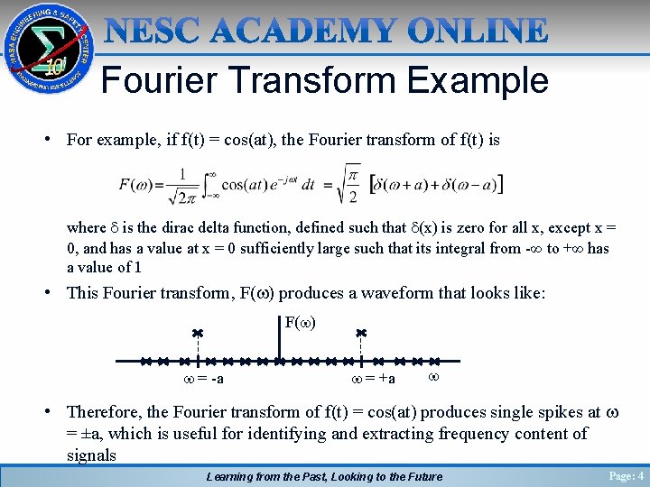
Fourier Transform Example • For example, if f(t) = cos(at), the Fourier transform of f(t) is where d is the dirac delta function, defined such that d(x) is zero for all x, except x = 0, and has a value at x = 0 sufficiently large such that its integral from -∞ to +∞ has a value of 1 • This Fourier transform, F(w) produces a waveform that looks like: F(w) w = -a w = +a w • Therefore, the Fourier transform of f(t) = cos(at) produces single spikes at w = ±a, which is useful for identifying and extracting frequency content of signals Learning from the Past, Looking to the Future Page: 4

• Linearity Property of Fourier Transform Now, if f(t) is composed of many sinusoids, the linearity property of the Fourier transform requires that the Fourier transform of f(t) will have discrete non-zero spikes at each distinct frequency of those sinusoids. This is the essential property of Fourier analysis that is key to signal processing. For example, if ʄ { } represents the Fourier transform shown earlier, then – Linearity property of Fourier transforms: ʄ { a · f(t) + b · g(t) } a · F(w) + b · G(w) – Convolution property of Fourier transforms (* denotes convolution, • denotes ordinary multiplication): ʄ { f(t) * g(t) } √ 2π · [ F(w) · G(w) ] – Multiplication property of Fourier transforms: ʄ { f(t) · g(t) } 1/(√ 2π) · [ F(w) * G(w) ] – That is, multiplication in the time domain is convolution in the frequency domain, and vice-versa Learning from the Past, Looking to the Future Page: 5

Convolution - Definition • Convolution is a mathematical operator, acting on two functions, which computes the integral of the product of the two functions where one is reversed and shifted in its independent variable – Note that the asterisk (*) is typically used to denote convolution – The range of integration, t = a to b, depends on the domain over which the functions f and g are defined • Discrete convolution of sequences of “N” samples of functions f and g is computed by: Learning from the Past, Looking to the Future Page: 6

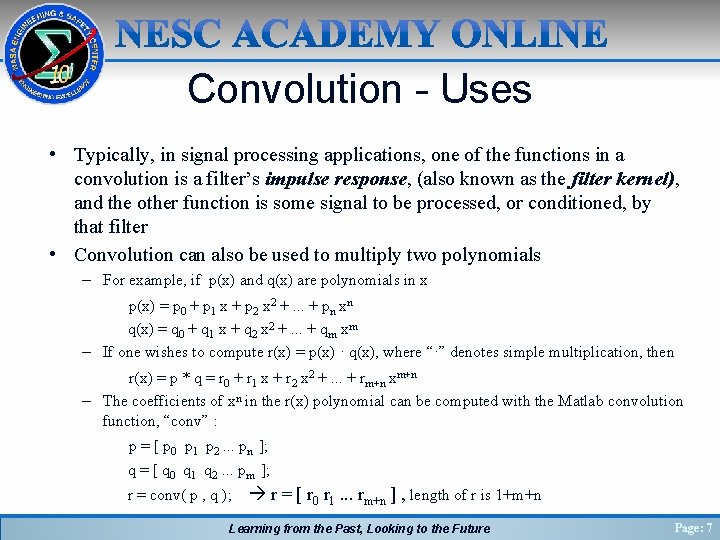
Convolution - Uses • Typically, in signal processing applications, one of the functions in a convolution is a filter’s impulse response, (also known as the filter kernel), and the other function is some signal to be processed, or conditioned, by that filter • Convolution can also be used to multiply two polynomials – For example, if p(x) and q(x) are polynomials in x p(x) = p 0 + p 1 x + p 2 x 2 +. . . + pn xn q(x) = q 0 + q 1 x + q 2 x 2 +. . . + qm xm – If one wishes to compute r(x) = p(x) · q(x), where “·” denotes simple multiplication, then r(x) = p * q = r 0 + r 1 x + r 2 x 2 +. . . + rm+n xm+n – The coefficients of xn in the r(x) polynomial can be computed with the Matlab convolution function, “conv” : p = [ p 0 p 1 p 2. . . pn ]; q = [ q 0 q 1 q 2. . . pm ]; r = conv( p , q ); r = [ r 0 r 1. . . rm+n ] , length of r is 1+m+n Learning from the Past, Looking to the Future Page: 7

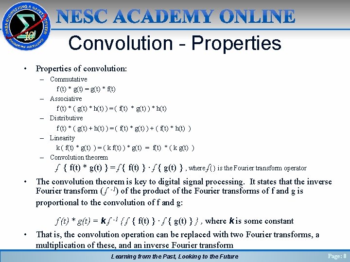
Convolution - Properties • Properties of convolution: – Commutative f (t) * g(t) = g(t) * f(t) – Associative f (t) * ( g(t) * h(t) ) = ( f(t) * g(t) ) * h(t) – Distributive f (t) * ( g(t) + h(t) ) = ( f(t) * g(t) ) + ( f(t) * h(t) ) – Linearity k ( f(t) * g(t) ) = ( k f(t) ) * g(t) = f(t) * ( k g(t) ) – Convolution theorem ʄ { f(t) * g(t) } = ʄ { f(t) } · ʄ { g(t) } , where ʄ{} is the Fourier transform operator • The convolution theorem is key to digital signal processing. It states that the inverse Fourier transform ( ʄ -1) of the product of the Fourier transforms of f and g is proportional to the convolution of f and g: f (t) * g(t) = k ʄ • -1 { ʄ { f(t) } · ʄ { g(t) } } , where k is some constant That is, the convolution operation can be replaced with two Fourier transforms, a multiplication of these, and an inverse Fourier transform Learning from the Past, Looking to the Future Page: 8

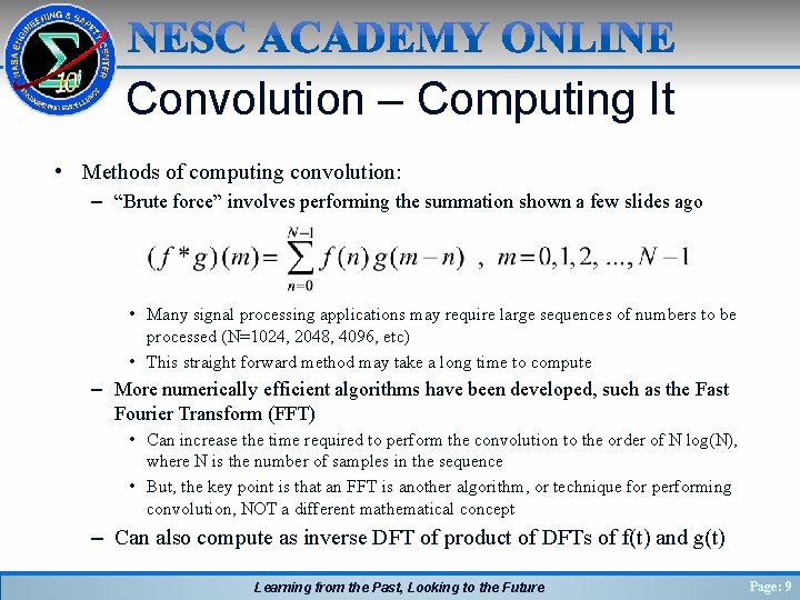
Convolution – Computing It • Methods of computing convolution: – “Brute force” involves performing the summation shown a few slides ago • Many signal processing applications may require large sequences of numbers to be processed (N=1024, 2048, 4096, etc) • This straight forward method may take a long time to compute – More numerically efficient algorithms have been developed, such as the Fast Fourier Transform (FFT) • Can increase the time required to perform the convolution to the order of N log(N), where N is the number of samples in the sequence • But, the key point is that an FFT is another algorithm, or technique for performing convolution, NOT a different mathematical concept – Can also compute as inverse DFT of product of DFTs of f(t) and g(t) Learning from the Past, Looking to the Future Page: 9

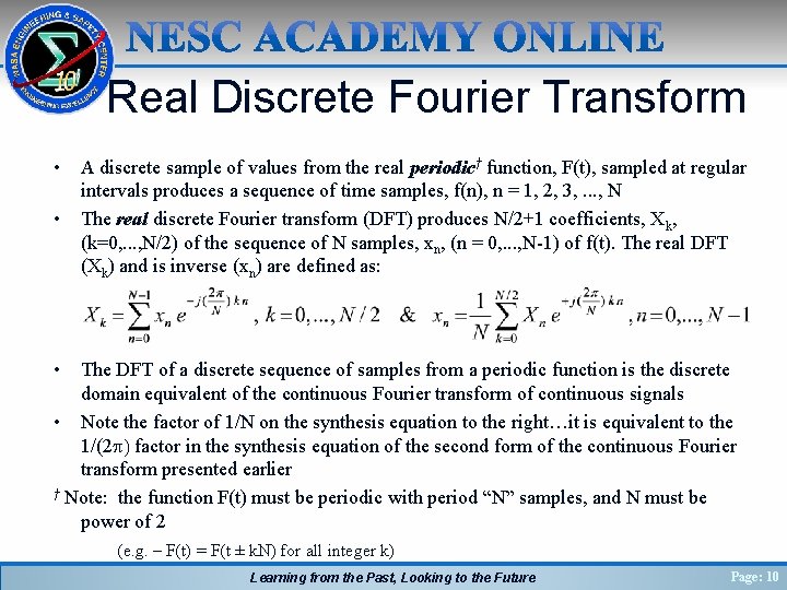
Real Discrete Fourier Transform • • A discrete sample of values from the real periodic† function, F(t), sampled at regular intervals produces a sequence of time samples, f(n), n = 1, 2, 3, . . . , N The real discrete Fourier transform (DFT) produces N/2+1 coefficients, Xk, (k=0, . . . , N/2) of the sequence of N samples, xn, (n = 0, . . . , N-1) of f(t). The real DFT (Xk) and is inverse (xn) are defined as: • The DFT of a discrete sequence of samples from a periodic function is the discrete domain equivalent of the continuous Fourier transform of continuous signals • Note the factor of 1/N on the synthesis equation to the right…it is equivalent to the 1/(2 p) factor in the synthesis equation of the second form of the continuous Fourier transform presented earlier † Note: the function F(t) must be periodic with period “N” samples, and N must be power of 2 (e. g. – F(t) = F(t ± k. N) for all integer k) Learning from the Past, Looking to the Future Page: 10

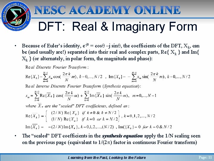
DFT: Real & Imaginary Form • Because of Euler’s identity, e-jq = cosq –j sinq, the coefficients of the DFT, Xk, can be (and usually are!) separated into their real and complex parts, Re{ Xk } and Im{ Xk } (or alternately, in polar form, the magnitude and phase): • The “scaled” DFT coefficients in the synthesis equation apply the 1/N scaling seen on the previous page (equivalent to 1/(2 p) factor in continuous Fourier transform) Learning from the Past, Looking to the Future Page: 11

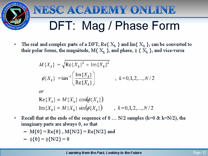
DFT: Mag / Phase Form • The real and complex parts of a DFT, Re{ Xk } and Im{ Xk }, can be converted to their polar forms, the magnitude, M{ Xk }, and phase, f { Xk }, and vice-versa • Recall that at the ends of the sequence of 0 … N/2 samples (k=0 & k=N/2), the imaginary parts are always 0, so that – M{0} = Re{0} , M{N/2} = Re{N/2} and – f{0} = f{N/2} = 0 Learning from the Past, Looking to the Future Page: 12

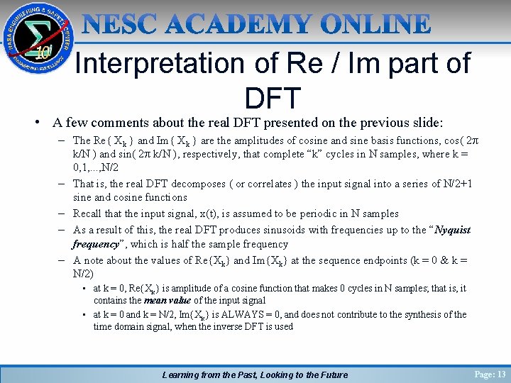
Interpretation of Re / Im part of DFT • A few comments about the real DFT presented on the previous slide: – The Re{ Xk } and Im{ Xk } are the amplitudes of cosine and sine basis functions, cos( 2 p k/N ) and sin( 2 p k/N ), respectively, that complete “k” cycles in N samples, where k = 0, 1, . . . , N/2 – That is, the real DFT decomposes ( or correlates ) the input signal into a series of N/2+1 sine and cosine functions – Recall that the input signal, x(t), is assumed to be periodic in N samples – As a result of this, the real DFT produces sinusoids with frequencies up to the “Nyquist frequency”, which is half the sample frequency – A note about the values of Re{Xk} and Im{Xk} at the sequence endpoints (k = 0 & k = N/2) • at k = 0, Re{Xk} is amplitude of a cosine function that makes 0 cycles in N samples; that is, it contains the mean value of the input signal • at k = 0 and k = N/2, Im{Xk} is ALWAYS = 0, and does not contribute to the synthesis of the time domain signal, when the inverse DFT is used Learning from the Past, Looking to the Future Page: 13

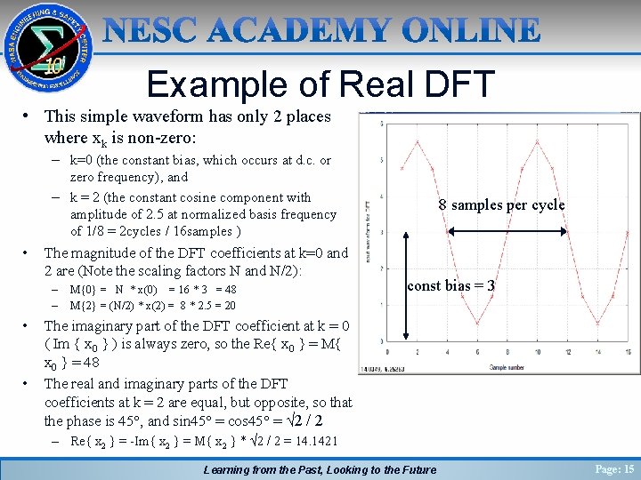
Example of Real DFT • Consider a 16 sample waveform, composed of a 2. 5 unit amplitude sine function completing two cycles in its 16 samples, with a constant bias of 3 units: 8 samples per cycle amp = 2. 5 (units) , bias = 3. 0 (units) , f = 2 cycles in N = 16 samples ( 8 samples/cycle ) xi = bias + amp * sin( 2 p * f * i / N ) , i = 1, 2, . . . , N • Compute the 16 -point real DFT of x in rectangular { Re , Im } form: const bias = 3 [ Re , Im , freq ] = dft_fft( x , 16 , 0 ); • Compute the 16 -point real DFT of x in polar { mag , phase } form: [ mag , phase , freq ] = dft_fft( x , 16 , 1 ); Learning from the Past, Looking to the Future Page: 14

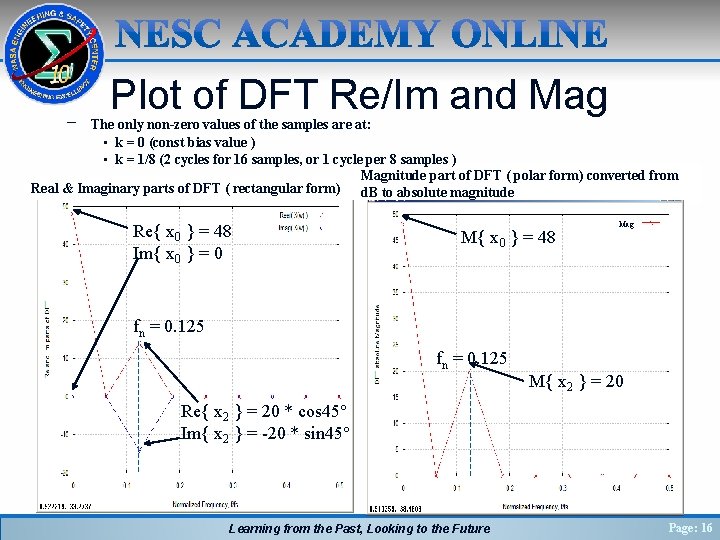
Example of Real DFT • This simple waveform has only 2 places where xk is non-zero: • – k=0 (the constant bias, which occurs at d. c. or zero frequency), and – k = 2 (the constant cosine component with amplitude of 2. 5 at normalized basis frequency of 1/8 = 2 cycles / 16 samples ) The magnitude of the DFT coefficients at k=0 and 2 are (Note the scaling factors N and N/2): – M{0} = N * x(0) = 16 * 3 = 48 – M{2} = (N/2) * x(2) = 8 * 2. 5 = 20 • • 8 samples per cycle const bias = 3 The imaginary part of the DFT coefficient at k = 0 ( Im { x 0 } ) is always zero, so the Re{ x 0 } = M{ x 0 } = 48 The real and imaginary parts of the DFT coefficients at k = 2 are equal, but opposite, so that the phase is 45°, and sin 45° = cos 45° = √ 2 / 2 – Re{ x 2 } = -Im{ x 2 } = M{ x 2 } * √ 2 / 2 = 14. 1421 Learning from the Past, Looking to the Future Page: 15

− Plot of DFT Re/Im and Mag The only non-zero values of the samples are at: • k = 0 (const bias value ) • k = 1/8 (2 cycles for 16 samples, or 1 cycle per 8 samples ) Magnitude part of DFT ( polar form) converted from Real & Imaginary parts of DFT ( rectangular form) d. B to absolute magnitude Re{ x 0 } = 48 Im{ x 0 } = 0 M{ x 0 } = 48 Mag fn = 0. 125 M{ x 2 } = 20 Re{ x 2 } = 20 * cos 45° Im{ x 2 } = -20 * sin 45° Learning from the Past, Looking to the Future Page: 16

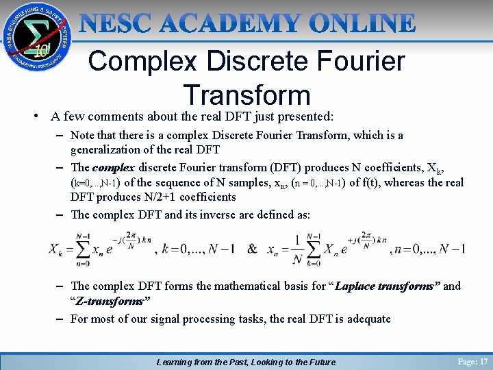
Complex Discrete Fourier Transform • A few comments about the real DFT just presented: – Note that there is a complex Discrete Fourier Transform, which is a generalization of the real DFT – The complex discrete Fourier transform (DFT) produces N coefficients, Xk, (k=0, . . . , N-1) of the sequence of N samples, xn, (n = 0, . . . , N-1) of f(t), whereas the real DFT produces N/2+1 coefficients – The complex DFT and its inverse are defined as: – The complex DFT forms the mathematical basis for “Laplace transforms” and “Z-transforms” – For most of our signal processing tasks, the real DFT is adequate Learning from the Past, Looking to the Future Page: 17

DFT – Requires Periodicity of input sequence • As a consequence of the requirement that the input sequence for a DFT must be samples from a periodic function, F(t), sampled at regular intervals, DFT does have limitations. Namely: – The DFT can only be represented for periodic signals, or finite duration signals – The inverse DFT cannot reproduce the entire time domain signal for non-periodic functions • But, fortunately, many of the waveforms that we are interested in are indeed periodic, or we are only interested in a finite length sequence of samples, so DFTs are an important signal processing tool Learning from the Past, Looking to the Future Page: 18

Fast Fourier Transform Algorithm • As mentioned earlier, the Fast Fourier Transform, or FFT, is a numerically efficient algorithm for computing the discrete Fourier transform, or DFT – FFT is NOT another mathematical concept, but a specific implementation method to compute DFTs efficiently – FFT can increase the speed of computing DFTs by order N log(N), where N is the number of samples of the signal being transformed – Many analysis packages, such as Matlab or Octave, include built in FFT functions • In Part 2 of this presentation “Power Spectral Density Basics”, we will discuss the Power Spectral Density techniques for analyzing spectral content of data, and will contrast it with the processing technique called the FFT which is used for more efficient calculations of DFTs needed for PSD analysis Learning from the Past, Looking to the Future Page: 19

Shannon Sampling Theorem & Data Aliasing • Shannon sampling theorem (paraphrased) – If a continuous signal is sampled at a frequency at least twice the frequency of the signal’s highest frequency content, the digitized samples can be used to completely reconstruct the original continuous signal • That is, if the signal being sampled contains no frequencies above the Nyquist frequency (half the sample frequency), its frequency content is preserved so that inverse DFT can be used to re-construct the original continuous signal • If the signal being sampled DOES contain frequencies above the Nyquist frequency, the frequency content of the signal above the Nyquist frequency will be “aliased”, or wrapped down into the lower frequency range (0 to 0. 5 normalized frequency, f/fs) as if a lower frequency content was present (and its power at that fictitious frequency will combine with any “real” signal content at that frequency) – Usually sampled data systems use “anti-aliasing” low pass filters to attenuate any signal above the Nyquist frequency so that anti-aliasing cannot occur Learning from the Past, Looking to the Future Page: 20

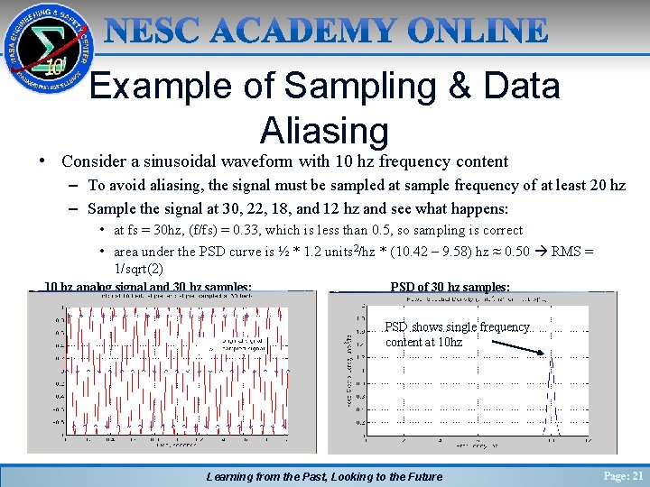
Example of Sampling & Data Aliasing • Consider a sinusoidal waveform with 10 hz frequency content – To avoid aliasing, the signal must be sampled at sample frequency of at least 20 hz – Sample the signal at 30, 22, 18, and 12 hz and see what happens: • at fs = 30 hz, (f/fs) = 0. 33, which is less than 0. 5, so sampling is correct • area under the PSD curve is ½ * 1. 2 units 2/hz * (10. 42 – 9. 58) hz ≈ 0. 50 RMS = 1/sqrt(2) 10 hz analog signal and 30 hz samples: PSD of 30 hz samples: PSD shows single frequency content at 10 hz Learning from the Past, Looking to the Future Page: 21

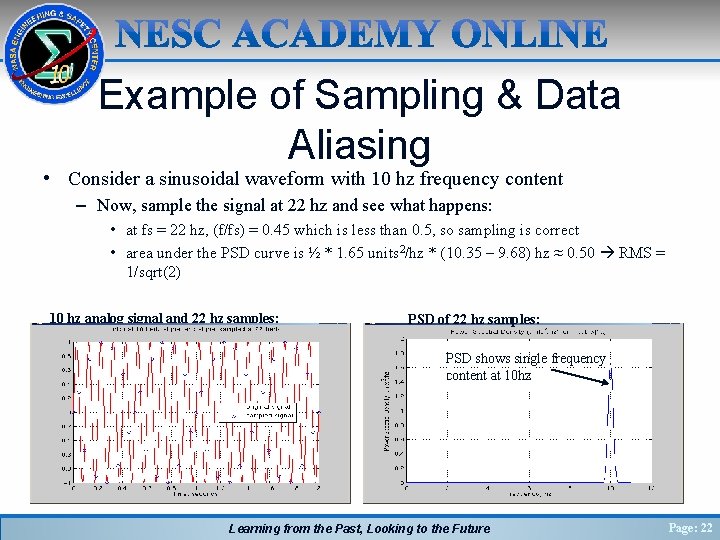
Example of Sampling & Data Aliasing • Consider a sinusoidal waveform with 10 hz frequency content – Now, sample the signal at 22 hz and see what happens: • at fs = 22 hz, (f/fs) = 0. 45 which is less than 0. 5, so sampling is correct • area under the PSD curve is ½ * 1. 65 units 2/hz * (10. 35 – 9. 68) hz ≈ 0. 50 RMS = 1/sqrt(2) 10 hz analog signal and 22 hz samples: PSD of 22 hz samples: PSD shows single frequency content at 10 hz Learning from the Past, Looking to the Future Page: 22

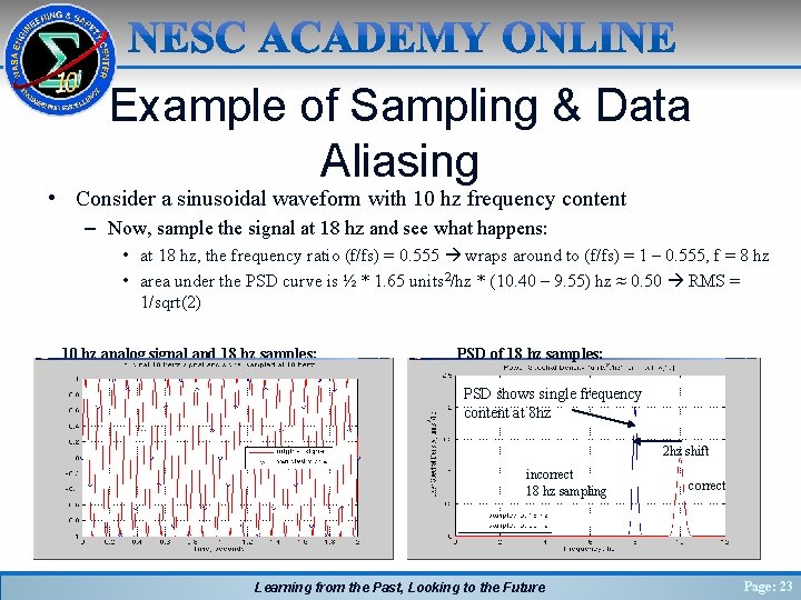
Example of Sampling & Data Aliasing • Consider a sinusoidal waveform with 10 hz frequency content – Now, sample the signal at 18 hz and see what happens: • at 18 hz, the frequency ratio (f/fs) = 0. 555 wraps around to (f/fs) = 1 – 0. 555, f = 8 hz • area under the PSD curve is ½ * 1. 65 units 2/hz * (10. 40 – 9. 55) hz ≈ 0. 50 RMS = 1/sqrt(2) 10 hz analog signal and 18 hz samples: PSD of 18 hz samples: PSD shows single frequency content at 8 hz 2 hz shift incorrect 18 hz sampling Learning from the Past, Looking to the Future correct Page: 23

Example of Sampling & Data Aliasing • Consider a sinusoidal waveform with 10 hz frequency content – Now, sample the signal at 12 hz and see what happens: • at 12 hz, the frequency ratio (f/fs) = 0. 833 wraps around to (f/fs) = 1 - 0. 833 f = 2 hz • area under the PSD curve is ½ * 3. 0 units 2/hz * (2. 15 – 1. 83) hz ≈ 0. 50 RMS = 1/sqrt(2) 10 hz analog signal and 12 hz samples: PSD of 12 hz samples: incorrect 12 hz sampling 8 hz shift correct Learning from the Past, Looking to the Future Page: 24

Introduction to DSP, Part 1 of 4 Summary • In Part 1, “Mathematical Concepts” we have covered the following: – Definitions, mathematical pre-requisites, and application techniques • Fourier transforms and convolution • Discrete Fourier transforms (DFT) and Fast Fourier transforms (FFT) • Shannon Sampling Theorem and data aliasing • In Part 2, “Power Spectral Density Basics”, we will cover the following: – Power Spectral Density (PSD) to estimate spectral characteristics of waveforms – PSD Demonstration • In Part 3 “Implementing Discrete Filters” we will cover the following: – Converting from continuous Laplace domain filters to discrete Z-domain filters (Tustin’s rule, or bilinear transformation) – Recursive filter implementations for discrete filters • In Part 4 “Typical GN&C Applications” we will cover the following: – – – Normalized frequency Methods to verify transfer function magnitude/phase of discrete filters using DFT (or FFT) Example use of discrete filter to implement a notch filter Learning from the Past, Looking to the Future Page: 25