Introduction to Digital Signal Processing DSP By Assoc

Introduction to Digital Signal Processing (DSP) By: Assoc. Prof. Dr. Erhan A. İnce Electrical and Electronic Engineering Dept. SPRING 2016 e-mail: erhan. ince@emu. edu. tr http: //faraday. ee. emu. edu. tr/eeng 420 1

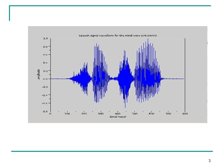
Digital Signal Processing And Its Benefits By a signal we mean any variable that carries or contains some kind of information that can be conveyed, displayed or manipulated. Examples of signals of particular interest to us engineers include: - Speech (encountered in telephony, radio, and everyday life ) 2

3

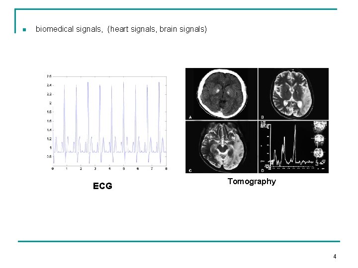
n biomedical signals, (heart signals, brain signals) ECG Tomography 4

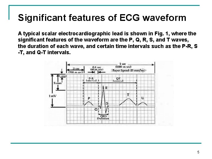
Significant features of ECG waveform A typical scalar electrocardiographic lead is shown in Fig. 1, where the significant features of the waveform are the P, Q, R, S, and T waves, the duration of each wave, and certain time intervals such as the P-R, S -T, and Q-T intervals. 5

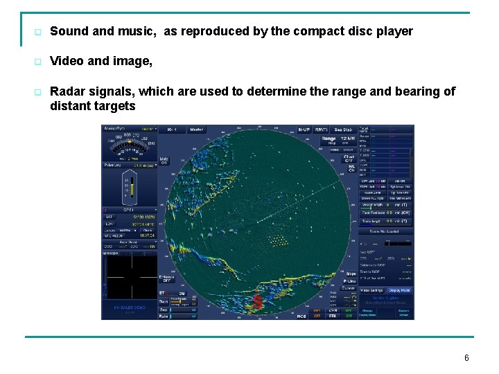
q Sound and music, as reproduced by the compact disc player q Video and image, q Radar signals, which are used to determine the range and bearing of distant targets 6

Ø Most of the signals in our environment are analog such as sound, temperature and light To processes these signals with a computer, we must: 1. convert the analog signals into electrical signals, e. g. , using a transducer such as a microphone to convert sound into electrical signal 2. digitize these signals, or convert them from analog to digital, using an ADC (Analog to Digital Converter) 7

Steps in Digital Signal Processing An analog input signal is filtered to be a band-limited signal by an input lowpass filter • Signal is then sampled and quantized by an ADC • Digital signal is processed by a digital circuit, often a computer or a digital signal processor • Processed digital signal is then converted back to an analog signal by a DAC • The resulting step waveform is converted to a smooth signal by a reconstruction filter called an anti-imaging filter 8

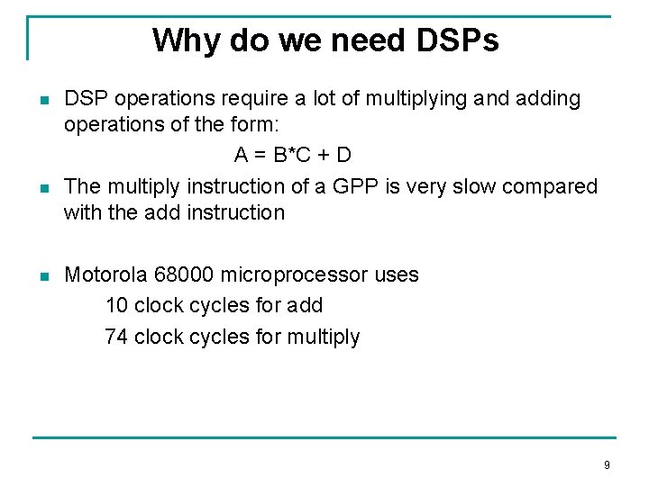
Why do we need DSPs n n n DSP operations require a lot of multiplying and adding operations of the form: A = B*C + D The multiply instruction of a GPP is very slow compared with the add instruction Motorola 68000 microprocessor uses 10 clock cycles for add 74 clock cycles for multiply 9

Digital signal processors can perform the multiply and the add operation in just one clock cycle Ø Most DSPs have a specialized instruction that causes them to multiply, add and save the result in a single cycle Ø This instruction is called a MAC (Multiply, Add, and Accumulate) Ø 10

Attraction of DSP comes from key advantages such as : * Guaranteed accuracy: (accuracy is only determined by the number of bits used) * Perfect Reproducibility: Identical performance from unit to unit ie. A digital recording can be copied or reproduced several times with no loss in signal quality * No drift in performance with temperature and age * Uses advances in semiconductor technology to achieve: (i) smaller size (ii) lower cost (iii) low power consumption (iv) higher operating speed * Greater flexibility: Reprogrammable , no need to modify the hardware * Superior performance ie. linear phase response can be achieved complex adaptive filtering becomes possible 11

Disadvantages of DSP * Speed and Cost DSP techniques are limited to signals with relatively low bandwidths DSP designs can be expensive, especially when large bandwidth signals are involved. ADC or DACs are either to expensive or do not have sufficient resolution for wide bandwidth applications. * DSP designs can be time consuming plus need the necessary resources (software etc) * Finite word-length problems If only a limited number of bits is used due to economic considerations serious degradation in system performance may result. 12

§ The use of finite precision arithmetic makes it necessary to quantize filter calculations by rounding or truncation. § Round-off noise is that error in the filter output that results from rounding or truncating calculations within the filter. § As the name implies, this error looks like low-level noise at the filter output 13

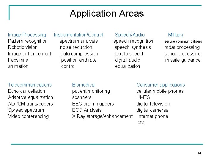
Application Areas Image Processing Instrumentation/Control Pattern recognition spectrum analysis Robotic vision noise reduction Image enhancement data compression Facsimile position and rate animation control Telecommunications Echo cancellation Adaptive equalization ADPCM trans-coders Spread spectrum Video conferencing Speech/Audio speech recognition speech synthesis text to speech digital audio equalization Biomedical patient monitoring scanners EEG brain mappers ECG Analysis X-Ray storage/enhancement Military secure communications radar processing sonar processing missile guidance Consumer applications cellular mobile phones UMTS digital television digital cameras internet phone etc. 14

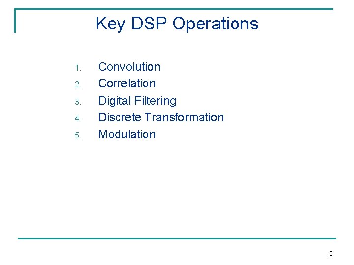
Key DSP Operations 1. 2. 3. 4. 5. Convolution Correlation Digital Filtering Discrete Transformation Modulation 15

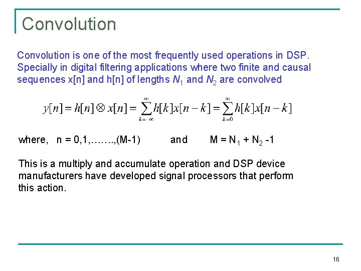
Convolution is one of the most frequently used operations in DSP. Specially in digital filtering applications where two finite and causal sequences x[n] and h[n] of lengths N 1 and N 2 are convolved where, n = 0, 1, ……. , (M-1) and M = N 1 + N 2 -1 This is a multiply and accumulate operation and DSP device manufacturers have developed signal processors that perform this action. 16

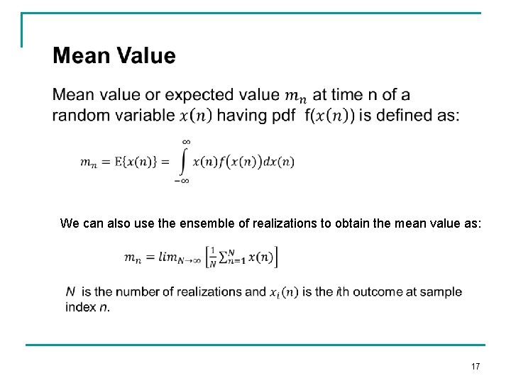
We can also use the ensemble of realizations to obtain the mean value as: 17

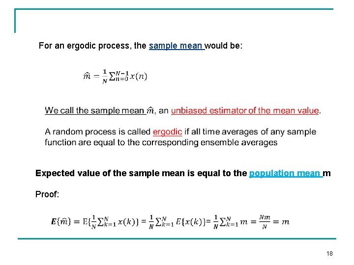
For an ergodic process, the sample mean would be: Expected value of the sample mean is equal to the population mean m Proof: 18

Correlation There are two forms of correlation : 1. Auto-correlation 2. Cross-correlation 19

Autocorrelation is a special case for cross-correlation Auto-covariance is a special case of cross-covariance. 20

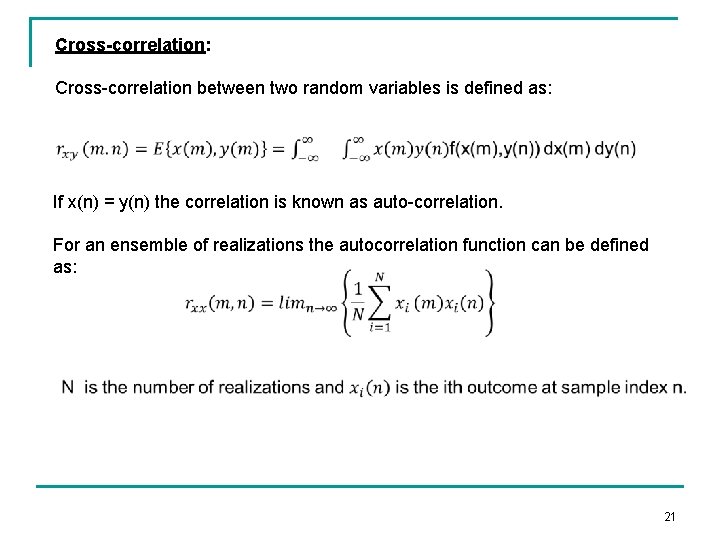
Cross-correlation: Cross-correlation between two random variables is defined as: If x(n) = y(n) the correlation is known as auto-correlation. For an ensemble of realizations the autocorrelation function can be defined as: 21

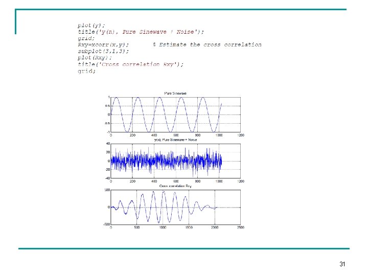
Cross-correlation is very useful in signal detection in which the interest is to find whether or not a desired signal exists in an observed (noisy)signal. 22

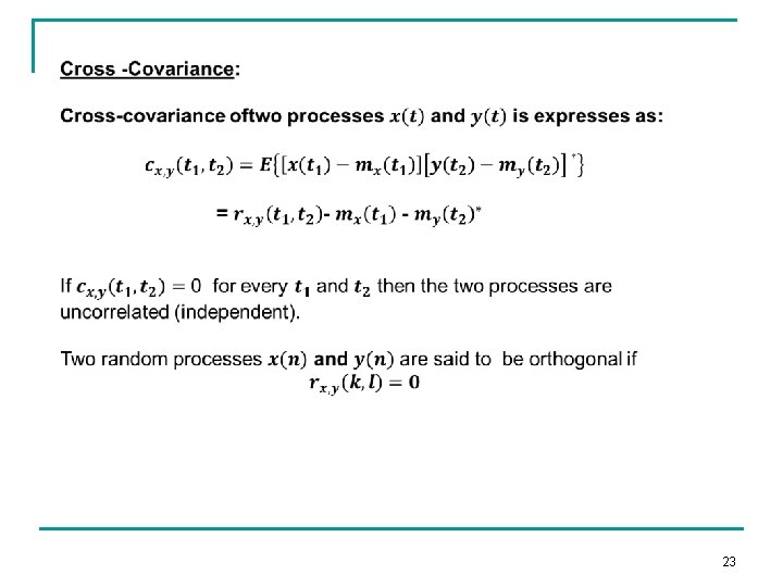
23

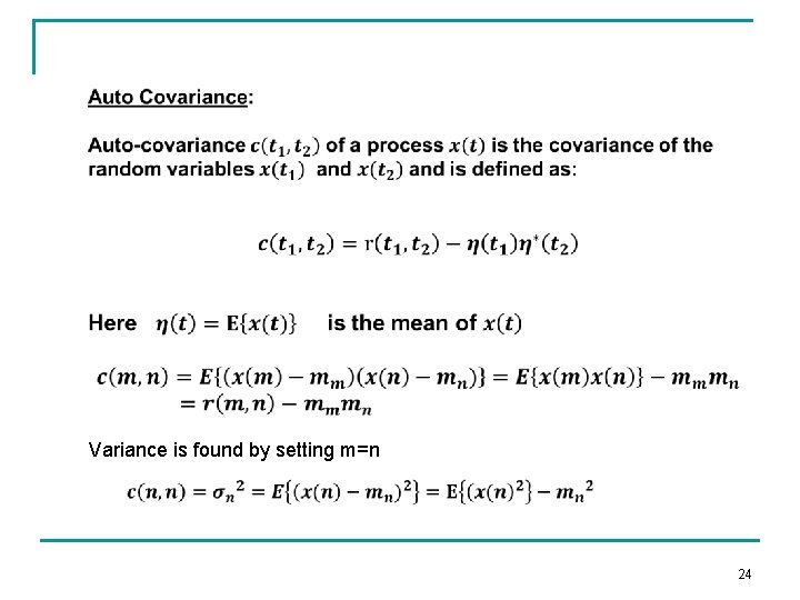
Variance is found by setting m=n 24

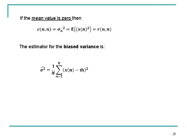
If the mean value is zero then The estimator for the biased variance is: 25

26

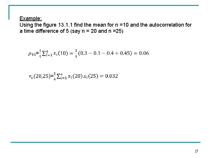
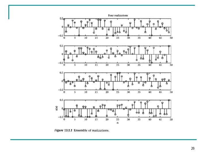
Example: Using the figure 13. 1. 1 find the mean for n =10 and the autocorrelation for a time difference of 5 (say n = 20 and n =25) 27

28

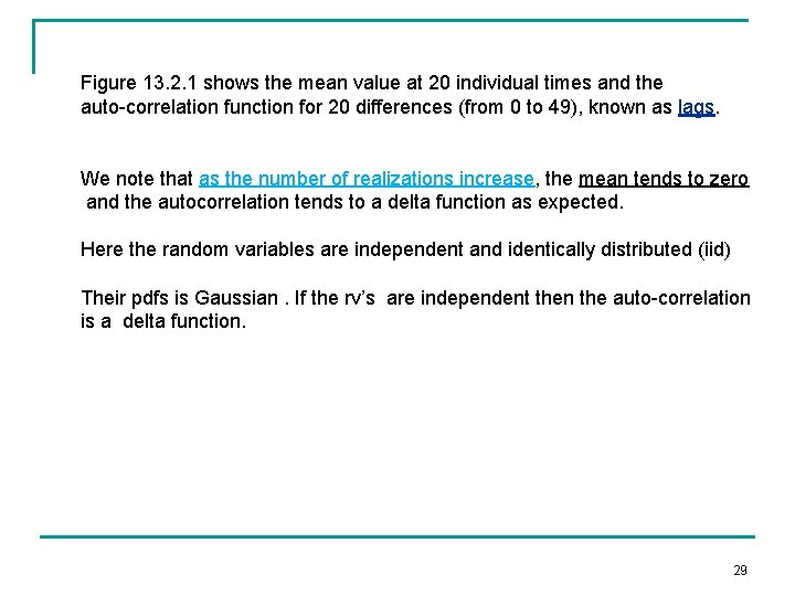
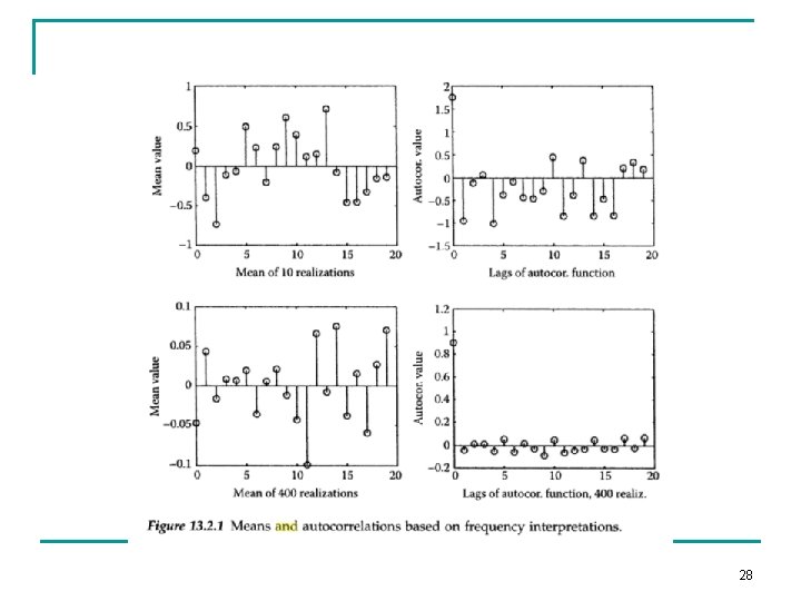
Figure 13. 2. 1 shows the mean value at 20 individual times and the auto-correlation function for 20 differences (from 0 to 49), known as lags. We note that as the number of realizations increase, the mean tends to zero and the autocorrelation tends to a delta function as expected. Here the random variables are independent and identically distributed (iid) Their pdfs is Gaussian. If the rv’s are independent then the auto-correlation is a delta function. 29

30

31

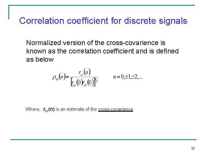
Correlation coefficient for discrete signals Normalized version of the cross-covarience is known as the correlation coefficient and is defined as below Where, rxy(n) is an estimate of the cross-covarience 32

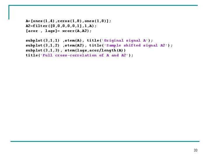
A=[ones(1, 4), zeros(1, 8), ones(1, 8)]; A 2=filter([0, 0, 0, 1], 1, A); [acor , lags]= xcorr(A, A 2); subplot(3, 1, 1) , stem(A), title('Original signal A'); subplot(3, 1, 2) , stem(A 2), title('Sample shifted signal A 2'); subplot(3, 1, 3), stem(lags, acor/length(A)) title('Full cross-correlation of A and A 2'); 33

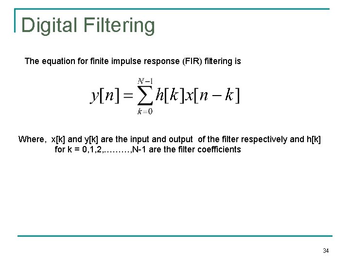
Digital Filtering The equation for finite impulse response (FIR) filtering is Where, x[k] and y[k] are the input and output of the filter respectively and h[k] for k = 0, 1, 2, ………, N-1 are the filter coefficients 34

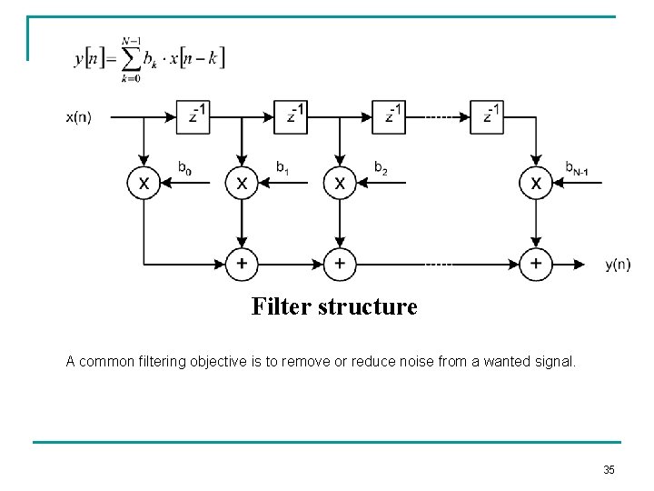
Filter structure A common filtering objective is to remove or reduce noise from a wanted signal. 35

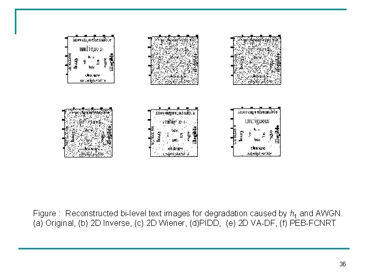
Figure : Reconstructed bi-level text images for degradation caused by h 1 and AWGN. (a) Original, (b) 2 D Inverse, (c) 2 D Wiener, (d)PIDD, (e) 2 D VA-DF, (f) PEB-FCNRT 36

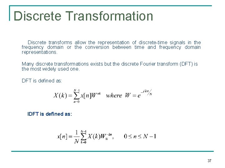
Discrete Transformation Discrete transforms allow the representation of discrete-time signals in the frequency domain or the conversion between time and frequency domain representations. Many discrete transformations exists but the discrete Fourier transform (DFT) is the most widely used one. DFT is defined as: IDFT is defined as: 37

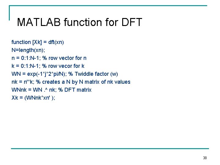
MATLAB function for DFT function [Xk] = dft(xn) N=length(xn); n = 0: 1: N-1; % row vector for n k = 0: 1: N-1; % row vecor for k WN = exp(-1*j*2*pi/N); % Twiddle factor (w) nk = n'*k; % creates a N by N matrix of nk values WNnk = WN. ^ nk; % DFT matrix Xk = (WNnk*xn' ); 38

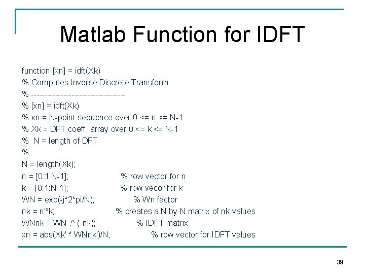
Matlab Function for IDFT function [xn] = idft(Xk) % Computes Inverse Discrete Transform % -----------------% [xn] = idft(Xk) % xn = N-point sequence over 0 <= n <= N-1 % Xk = DFT coeff. array over 0 <= k <= N-1 % N = length of DFT % N = length(Xk); n = [0: 1: N-1]; % row vector for n k = [0: 1: N-1]; % row vecor for k WN = exp(-j*2*pi/N); % Wn factor nk = n'*k; % creates a N by N matrix of nk values WNnk = WN. ^ (-nk); % IDFT matrix xn = abs(Xk' * WNnk')/N; % row vector for IDFT values 39

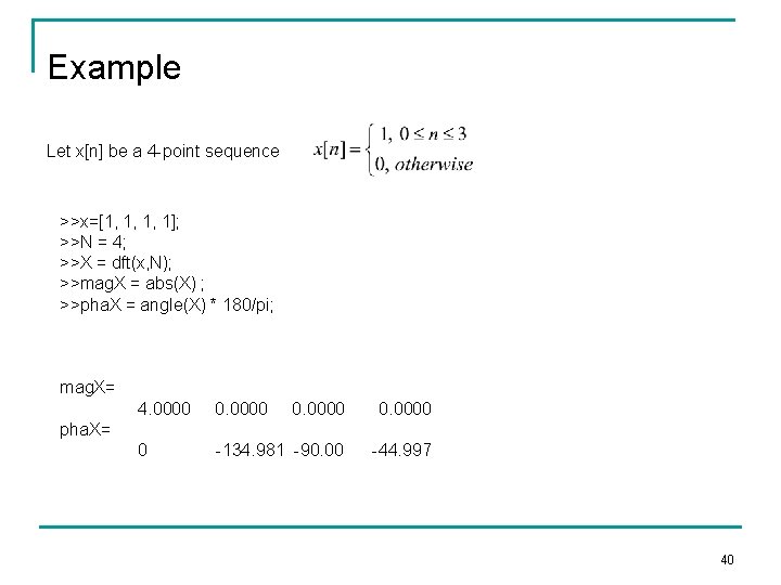
Example Let x[n] be a 4 -point sequence >>x=[1, 1, 1, 1]; >>N = 4; >>X = dft(x, N); >>mag. X = abs(X) ; >>pha. X = angle(X) * 180/pi; mag. X= 4. 0000 0 -134. 981 -90. 00 -44. 997 pha. X= 40

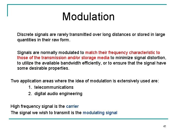
Modulation Discrete signals are rarely transmitted over long distances or stored in large quantities in their raw form. Signals are normally modulated to match their frequency characteristic to those of the transmission and/or storage media to minimize signal distortion, to utilize the available bandwidth efficiently, or to ensure that the signal have some desirable properties. Two application areas where the idea of modulation is extensively used are: 1. telecommunications 2. digital audio engineering High frequency signal is the carrier The signal we wish to transmit is the modulating signal 41

Three most commonly used digital modulation schemes for transmitting Digital data over bandpass channels are: Amplitude shift keying (ASK) Phase shift keying (PSK) Frequency shift keying (FSK) When digital data is transmitted over an all digital network a scheme known As pulse code modulation (PCM) is used. 42