Introduction to Digital Image Processing with MATLAB Asia
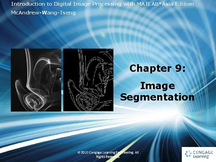
Introduction to Digital Image Processing with MATLAB® Asia Edition Mc. Andrew‧Wang‧Tseng Chapter 9: Image Segmentation 1 © 2010 Cengage Learning Engineering. All Rights Reserved. 1
9. 1 Introduction • Segmentation refers to the operation of partitioning an image into component parts or into separate objects • In this chapter, we will investigate two very important topics: thresholding and edge detection 2 Ch 9 -p. 221 © 2010 Cengage Learning Engineering. All Rights Reserved.
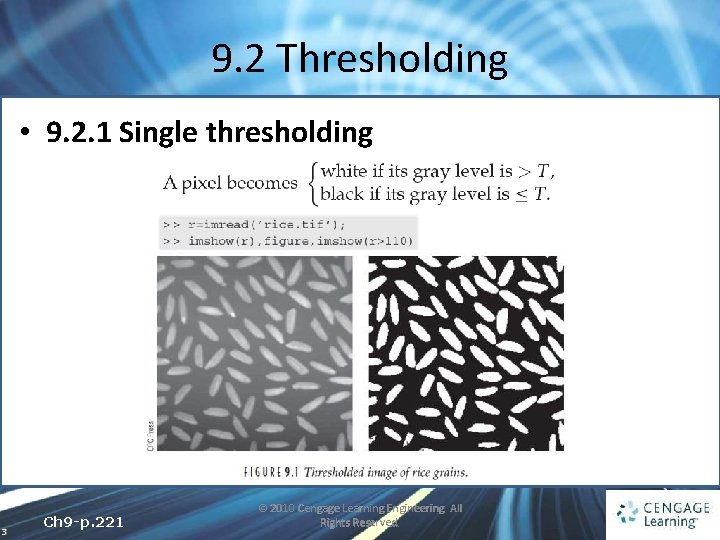
9. 2 Thresholding • 9. 2. 1 Single thresholding 3 Ch 9 -p. 221 © 2010 Cengage Learning Engineering. All Rights Reserved.
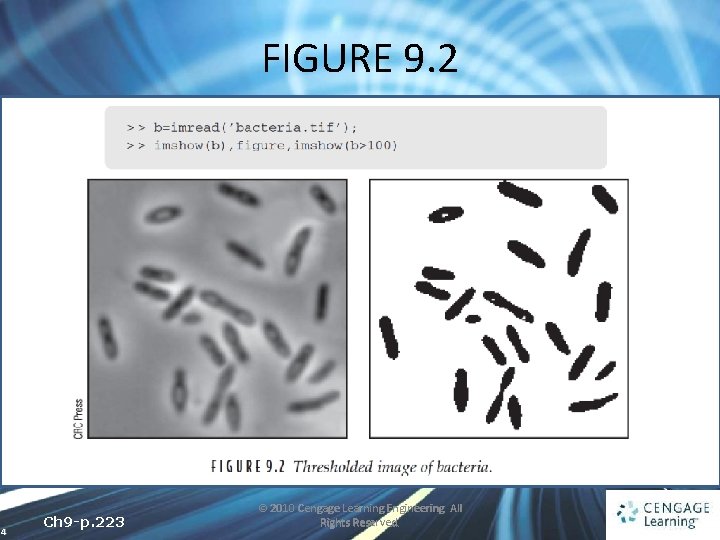
FIGURE 9. 2 4 Ch 9 -p. 223 © 2010 Cengage Learning Engineering. All Rights Reserved.
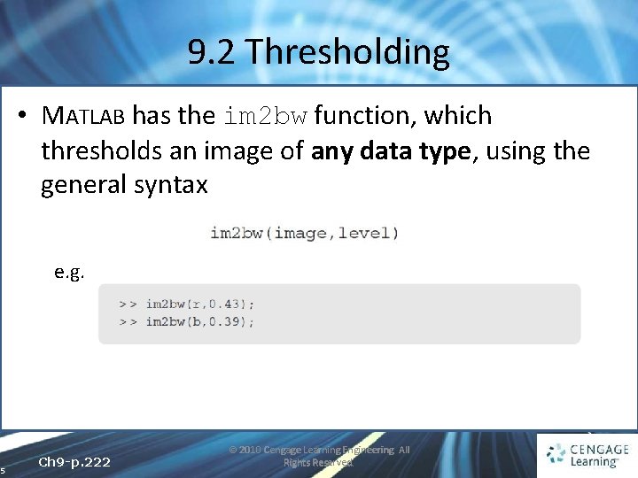
9. 2 Thresholding • MATLAB has the im 2 bw function, which thresholds an image of any data type, using the general syntax e. g. 5 Ch 9 -p. 222 © 2010 Cengage Learning Engineering. All Rights Reserved.

FIGURE 9. 3 • Showing hidden aspects of an image 6 Ch 9 -p. 223 © 2010 Cengage Learning Engineering. All Rights Reserved.
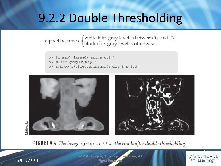
9. 2. 2 Double Thresholding 7 Ch 9 -p. 224 © 2010 Cengage Learning Engineering. All Rights Reserved.

9. 3 Applications of Thresholdng • Remove a varying background from text or a drawing 8 Ch 9 -p. 225 © 2010 Cengage Learning Engineering. All Rights Reserved.
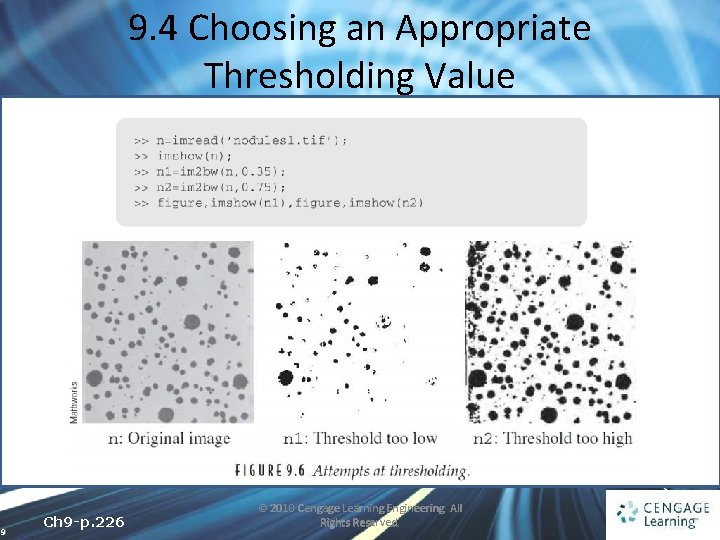
9. 4 Choosing an Appropriate Thresholding Value 9 Ch 9 -p. 226 © 2010 Cengage Learning Engineering. All Rights Reserved.

FIGURE 9. 7 10 Ch 9 -p. 227 © 2010 Cengage Learning Engineering. All Rights Reserved.

FIGURE 9. 8 • Describe the image histogram as a probability distribution 11 Ch 9 -p. 228 © 2010 Cengage Learning Engineering. All Rights Reserved.

9. 4 Choosing an Appropriate Thresholding Value • We would like to find k to maximize the difference between ω(k) and μ(k) Define the image average as then find a k, which maximizes 12 Ch 9 -p. 228 © 2010 Cengage Learning Engineering. All Rights Reserved. (Otsu’s method, MATLAB function graythresh)

9. 4 Choosing an Appropriate Thresholding Value 13 Ch 9 -p. 229 © 2010 Cengage Learning Engineering. All Rights Reserved.

FIGURE 9. 9 14 Ch 9 -p. 230 © 2010 Cengage Learning Engineering. All Rights Reserved.

9. 5 Adaptive Thresholding 15 Ch 9 -p. 230 © 2010 Cengage Learning Engineering. All Rights Reserved.

FIGURE 9. 11 16 Ch 9 -p. 232 © 2010 Cengage Learning Engineering. All Rights Reserved.

9. 5 Adaptive Thresholding 17 Ch 9 -p. 231 © 2010 Cengage Learning Engineering. All Rights Reserved.

FIGURE 9. 12 18 Ch 9 -p. 232 © 2010 Cengage Learning Engineering. All Rights Reserved.

9. 6 Edge Detection • The general MATLAB command for finding edges is 19 Ch 9 -p. 233 © 2010 Cengage Learning Engineering. All Rights Reserved.

9. 7 Derivatives and Edges • 9. 7. 1 Fundamental Definitions Ramp edge 20 Ch 9 -p. 234 step edge © 2010 Cengage Learning Engineering. All Rights Reserved. Ramp edge step edge

FIGURE 9. 15 21 Ch 9 -p. 235 © 2010 Cengage Learning Engineering. All Rights Reserved.

9. 7. 2 Some Edge Detection Filters • Prewitt filters 22 Ch 9 -p. 236 © 2010 Cengage Learning Engineering. All Rights Reserved.

FIGURE 9. 16 & 17 23 Ch 9 -p. 237 © 2010 Cengage Learning Engineering. All Rights Reserved.

FIGURE 9. 18 24 Ch 9 -p. 238 © 2010 Cengage Learning Engineering. All Rights Reserved.

FIGURE 9. 19 25 Ch 9 -p. 238 © 2010 Cengage Learning Engineering. All Rights Reserved.

9. 7. 2 Some Edge Detection Filters • Roberts cross-gradient filters • Sobel filters 26 Ch 9 -p. 239 © 2010 Cengage Learning Engineering. All Rights Reserved.

FIGURE 9. 20 27 Ch 9 -p. 240 © 2010 Cengage Learning Engineering. All Rights Reserved.

9. 8 Second Derivatives • 9. 8. 1 The Laplacian ü Isotropic filter ü Very sensitive to noise 28 Ch 9 -p. 241 © 2010 Cengage Learning Engineering. All Rights Reserved.

FIGURE 9. 21 29 Ch 9 -p. 241 © 2010 Cengage Learning Engineering. All Rights Reserved.

FIGURE 9. 22 30 Ch 9 -p. 242 © 2010 Cengage Learning Engineering. All Rights Reserved.

9. 8. 2 Zero Crossing • The position where the result of the filter changes sign • e. g. , consider the simple image given in Figure 9. 23(a) and the result after filtering with a Laplacian mask in Figure 9. 23(b) 31 Ch 9 -p. 243 © 2010 Cengage Learning Engineering. All Rights Reserved.

FIGURE 9. 23 32 Ch 9 -p. 243 © 2010 Cengage Learning Engineering. All Rights Reserved.

9. 8. 2 Zero Crossing • We define the zero crossings in such a filtered image to be pixels that satisfy either of the following: ü They have a negative gray value and are orthogonally adjacent to a pixel whose gray value is positive ü They have a value of zero and are between negativeand positive-valued pixels 33 Ch 9 -p. 243 © 2010 Cengage Learning Engineering. All Rights Reserved.

FIGURE 9. 24 34 Ch 9 -p. 244 © 2010 Cengage Learning Engineering. All Rights Reserved.

9. 8. 2 Zero Crossing • Marr-Hildreth method ü Smooth the image with a Gaussian filter ü Convolve the result with a Laplacian filter ü Find the zero crossings 35 Ch 9 -p. 244 © 2010 Cengage Learning Engineering. All Rights Reserved.

FIGURE 9. 25 36 Ch 9 -p. 244 © 2010 Cengage Learning Engineering. All Rights Reserved.

9. 9 The Canny Edge Detector ü Take our image x ü Create a one-dimensional Gaussian filter g ü Create a one-dimensional filter dg corresponding to the expression given in ü 4. Convolve g with dg to obtain gdg ü 5. Apply gdg to x producing x 1 ü 6. Apply gdg’ to x producing x 2 We can now form an edge image with 37 Ch 9 -p. 246 © 2010 Cengage Learning Engineering. All Rights Reserved.

FIGURE 9. 26 ü Non-maximum suppression interpolation 38 Ch 9 -p. 246 © 2010 Cengage Learning Engineering. All Rights Reserved. p

FIGURE 9. 27 39 Ch 9 -p. 247 © 2010 Cengage Learning Engineering. All Rights Reserved.

FIGURE 9. 28 ü Hysteresis thresholding 40 Ch 9 -p. 248 © 2010 Cengage Learning Engineering. All Rights Reserved.

FIGURE 9. 29 41 Ch 9 -p. 248 © 2010 Cengage Learning Engineering. All Rights Reserved.

FIGURE 9. 30 42 Ch 9 -p. 249 © 2010 Cengage Learning Engineering. All Rights Reserved.

9. 10 The Hough Transform 43 Ch 9 -p. 250 © 2010 Cengage Learning Engineering. All Rights Reserved.

FIGURE 9. 32 44 Ch 9 -p. 251 © 2010 Cengage Learning Engineering. All Rights Reserved.

FIGURE 9. 33 45 Ch 9 -p. 252 © 2010 Cengage Learning Engineering. All Rights Reserved.

9. 10 The Hough Transform • We cannot express a vertical line in the form y = mx+c, because m represents the gradient and a vertical line has infinite gradient • Any line can be described in terms of the two parameters r and θ ü r is the perpendicular distance from the line to the origin ü θ is the angle of the line’s perpendicular to the x axis 46 Ch 9 -p. 252 © 2010 Cengage Learning Engineering. All Rights Reserved.

FIGURE 9. 34 47 Ch 9 -p. 252 © 2010 Cengage Learning Engineering. All Rights Reserved.

FIGURE 9. 35 • If we discretize θ to use only four values: -45°, 0°, 45°, 90° 48 Ch 9 -p. 254 © 2010 Cengage Learning Engineering. All Rights Reserved.

9. 10 The Hough Transform • The accumulator array contains the number of times each value of (r, θ) appears in the above table 49 Ch 9 -p. 254 © 2010 Cengage Learning Engineering. All Rights Reserved.

FIGURE 9. 36 50 Ch 9 -p. 255 © 2010 Cengage Learning Engineering. All Rights Reserved.

9. 11 Implementing the Hough Transform in MATLAB ü Decide on a discrete set of values of θ and r to use ü Calculate for each foreground pixel (x, y) in the image the values of r = xcosθ + ysinθ for all of our chosen values of θ ü Create an accumulator array whose sizes are the numbers of angles θ and values r in our chosen discretizations from Step 1, and ü Step through all of our r values, updating the accumulator array as we go 51 Ch 9 -p. 255 © 2010 Cengage Learning Engineering. All Rights Reserved.

FIGURE 9. 37 • 9. 11. 1 Discretizing r and θ >> angles = [-90: 180]*pi/180; 52 Ch 9 -p. 256 © 2010 Cengage Learning Engineering. All Rights Reserved.

9. 11 Implementing the Hough Transform in MATLAB 9. 11. 2 Calculating the r Values ü If im is a binary image We can create a binary edge image by use of the edge function 9. 11. 3 Forming the Accumulator Array 53 Ch 9 -p. 257 © 2010 Cengage Learning Engineering. All Rights Reserved.

9. 11 Implementing the Hough Transform in MATLAB • 9. 11. 4 Updating the Accumulator Array 54 Ch 9 -p. 257 © 2010 Cengage Learning Engineering. All Rights Reserved.

FIGURE 9. 39 55 Ch 9 -p. 258 © 2010 Cengage Learning Engineering. All Rights Reserved.

FIGURE 9. 40 56 Ch 9 -p. 259 © 2010 Cengage Learning Engineering. All Rights Reserved.

FIGURE 9. 41 57 Ch 9 -p. 261 © 2010 Cengage Learning Engineering. All Rights Reserved.

FIGURE 9. 42 58 Ch 9 -p. 261 © 2010 Cengage Learning Engineering. All Rights Reserved.
- Slides: 58