Introduction to Digital Image Processing with MATLAB Asia
Introduction to Digital Image Processing with MATLAB® Asia Edition Mc. Andrew‧Wang‧Tseng Chapter 4: Point Processing 1 © 2010 Cengage Learning Engineering. All Rights Reserved. 1
4. 1 Introduction • Any image-processing operation transforms the gray values of the pixels. • Image-processing operations may be divided into three classes based on the information required to perform the transformation. 2 Ch 4 -p. 65 © 2010 Cengage Learning Engineering. All Rights Reserved.
4. 1 Introduction From the most complex to the simplest, they are as follows: • Transforms • Neighborhood processing • Point operations 3 Ch 4 -p. 65 -66 © 2010 Cengage Learning Engineering. All Rights Reserved.
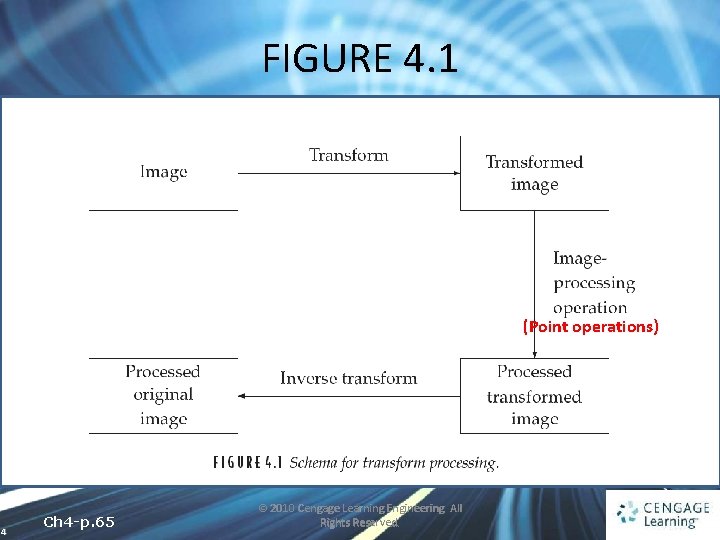
FIGURE 4. 1 (Point operations) 4 Ch 4 -p. 65 © 2010 Cengage Learning Engineering. All Rights Reserved.
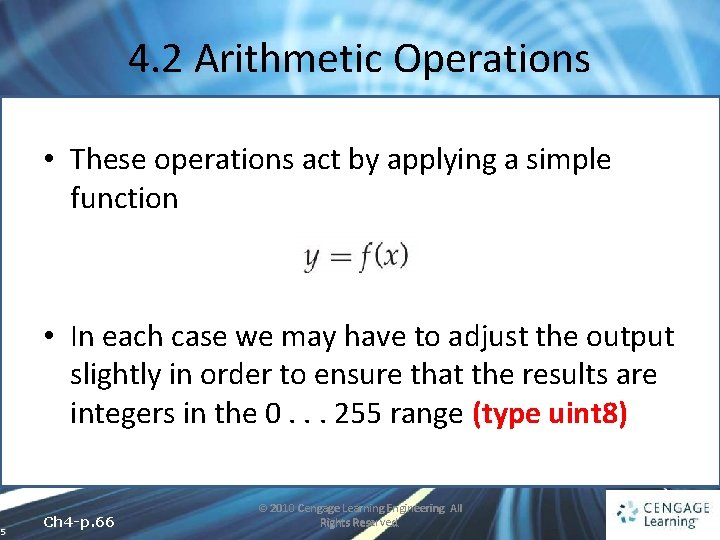
4. 2 Arithmetic Operations • These operations act by applying a simple function • In each case we may have to adjust the output slightly in order to ensure that the results are integers in the 0. . . 255 range (type uint 8) 5 Ch 4 -p. 66 © 2010 Cengage Learning Engineering. All Rights Reserved.
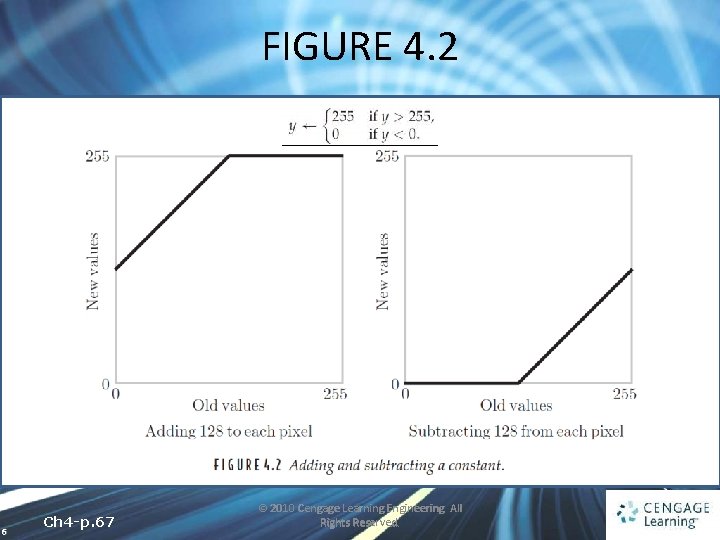
FIGURE 4. 2 6 Ch 4 -p. 67 © 2010 Cengage Learning Engineering. All Rights Reserved.
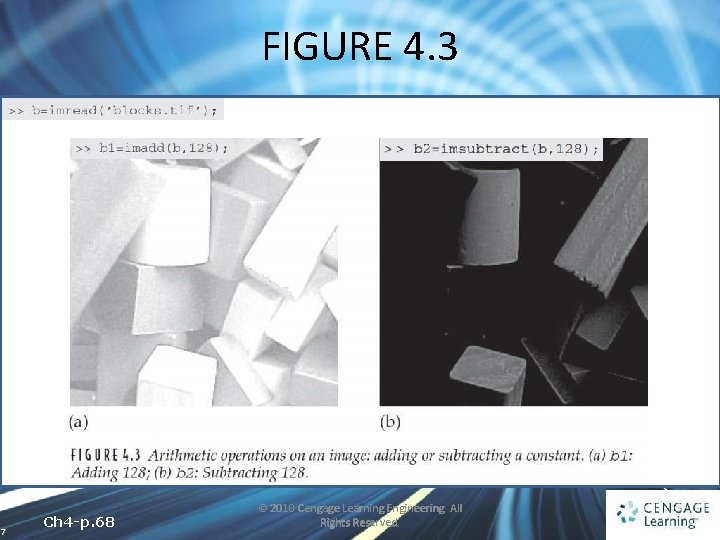
FIGURE 4. 3 7 Ch 4 -p. 68 © 2010 Cengage Learning Engineering. All Rights Reserved.
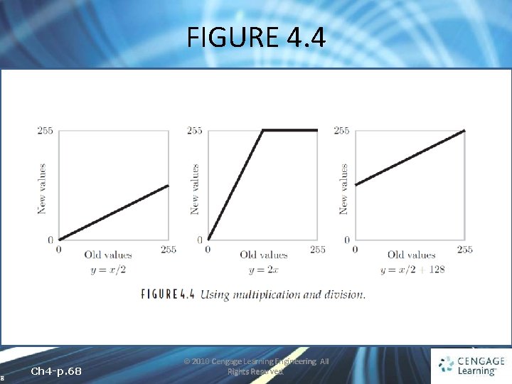
FIGURE 4. 4 8 Ch 4 -p. 68 © 2010 Cengage Learning Engineering. All Rights Reserved.
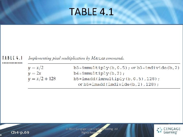
TABLE 4. 1 9 Ch 4 -p. 69 © 2010 Cengage Learning Engineering. All Rights Reserved.
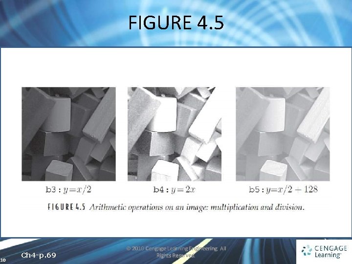
FIGURE 4. 5 10 Ch 4 -p. 69 © 2010 Cengage Learning Engineering. All Rights Reserved.
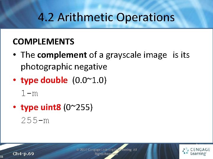
4. 2 Arithmetic Operations COMPLEMENTS • The complement of a grayscale image is its photographic negative • type double (0. 0~1. 0) 1 -m • type uint 8 (0~255) 255 -m 11 Ch 4 -p. 69 © 2010 Cengage Learning Engineering. All Rights Reserved.
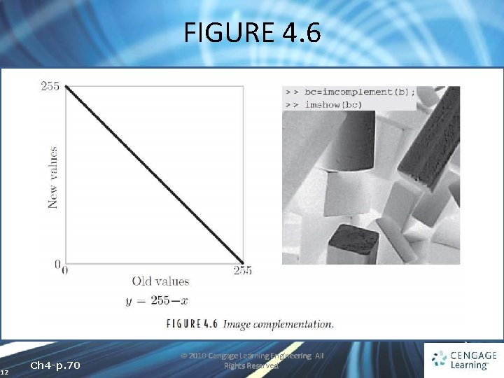
FIGURE 4. 6 12 Ch 4 -p. 70 © 2010 Cengage Learning Engineering. All Rights Reserved.
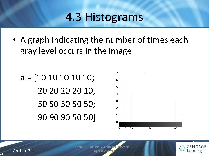
4. 3 Histograms • A graph indicating the number of times each gray level occurs in the image a = [10 10 10; 20 20 10; 50 50 50; 90 90 90 50 50] 13 Ch 4 -p. 71 © 2010 Cengage Learning Engineering. All Rights Reserved.
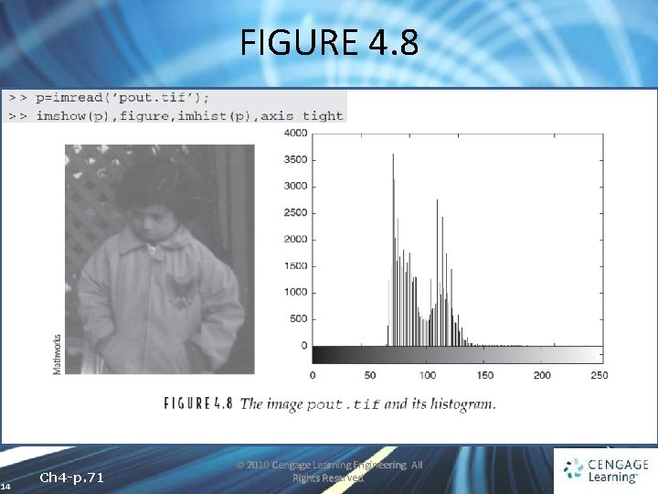
FIGURE 4. 8 14 Ch 4 -p. 71 © 2010 Cengage Learning Engineering. All Rights Reserved.
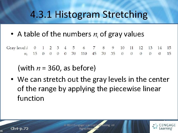
4. 3. 1 Histogram Stretching • A table of the numbers ni of gray values (with n = 360, as before) • We can stretch out the gray levels in the center of the range by applying the piecewise linear function 15 Ch 4 -p. 72 © 2010 Cengage Learning Engineering. All Rights Reserved.
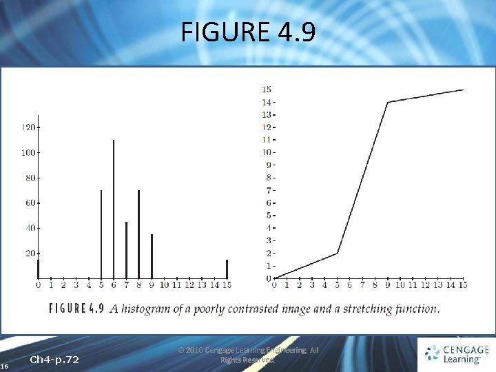
FIGURE 4. 9 16 Ch 4 -p. 72 © 2010 Cengage Learning Engineering. All Rights Reserved.
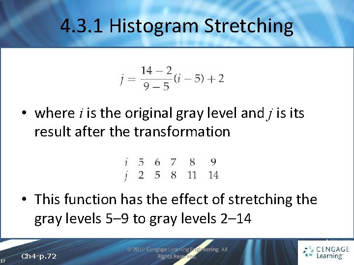
4. 3. 1 Histogram Stretching • where i is the original gray level and j is its result after the transformation • This function has the effect of stretching the gray levels 5– 9 to gray levels 2– 14 17 Ch 4 -p. 72 © 2010 Cengage Learning Engineering. All Rights Reserved.
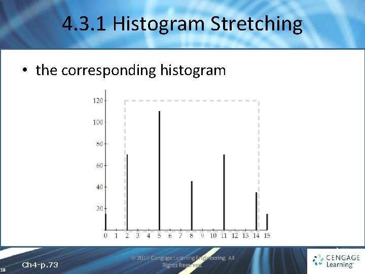
4. 3. 1 Histogram Stretching • the corresponding histogram 18 Ch 4 -p. 73 © 2010 Cengage Learning Engineering. All Rights Reserved.
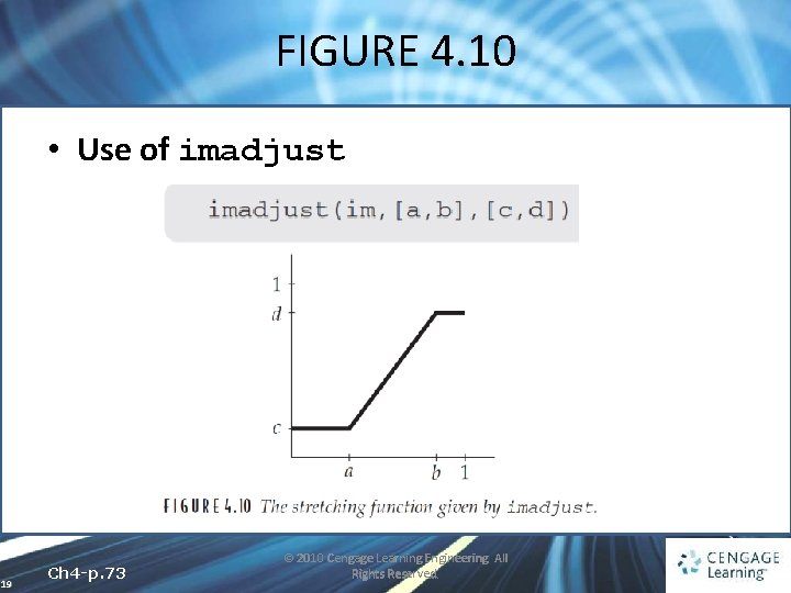
FIGURE 4. 10 • Use of imadjust 19 Ch 4 -p. 73 © 2010 Cengage Learning Engineering. All Rights Reserved.
4. 3. 1 Histogram Stretching • imadjust is designed to work equally well on images of type double, uint 8, or uint 16 • the values of a, b, c, and d must be between 0 and 1 • the function automatically converts the image im (if needed) to be of type double 20 Ch 4 -p. 73 © 2010 Cengage Learning Engineering. All Rights Reserved.
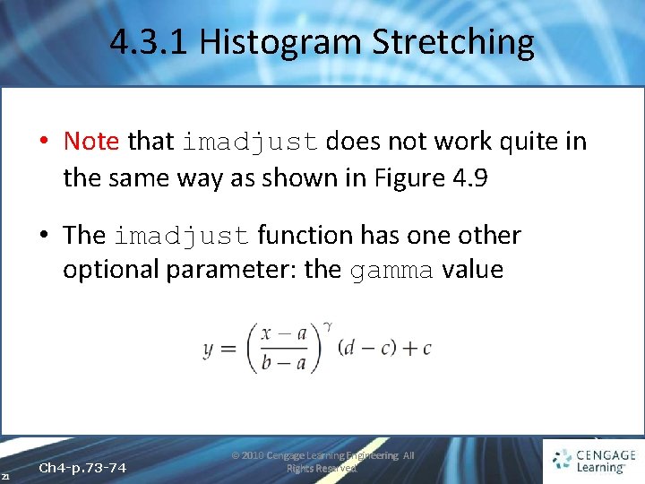
4. 3. 1 Histogram Stretching • Note that imadjust does not work quite in the same way as shown in Figure 4. 9 • The imadjust function has one other optional parameter: the gamma value 21 Ch 4 -p. 73 -74 © 2010 Cengage Learning Engineering. All Rights Reserved.
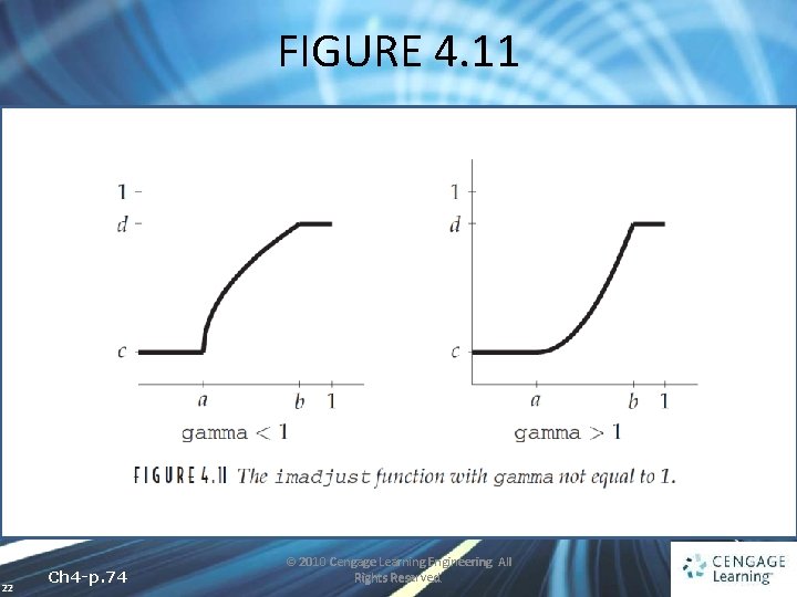
FIGURE 4. 11 22 Ch 4 -p. 74 © 2010 Cengage Learning Engineering. All Rights Reserved.
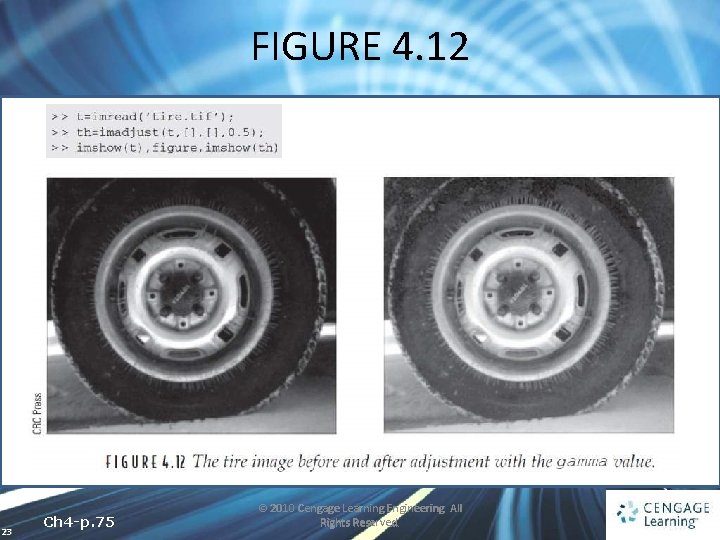
FIGURE 4. 12 23 Ch 4 -p. 75 © 2010 Cengage Learning Engineering. All Rights Reserved.
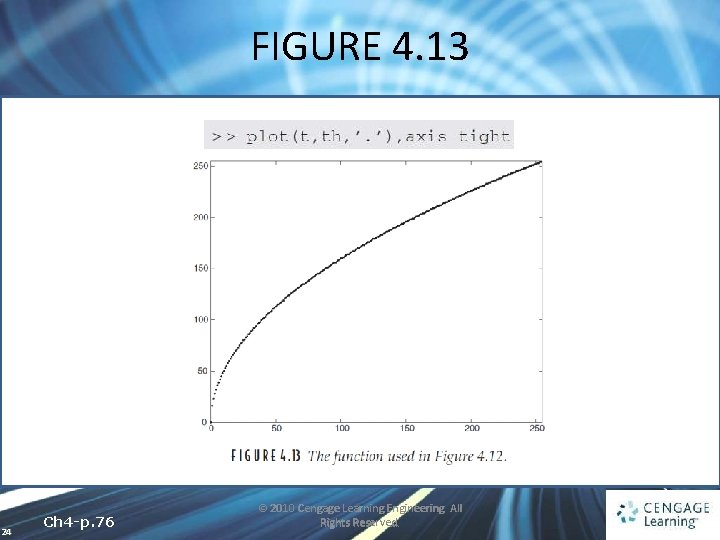
FIGURE 4. 13 24 Ch 4 -p. 76 © 2010 Cengage Learning Engineering. All Rights Reserved.
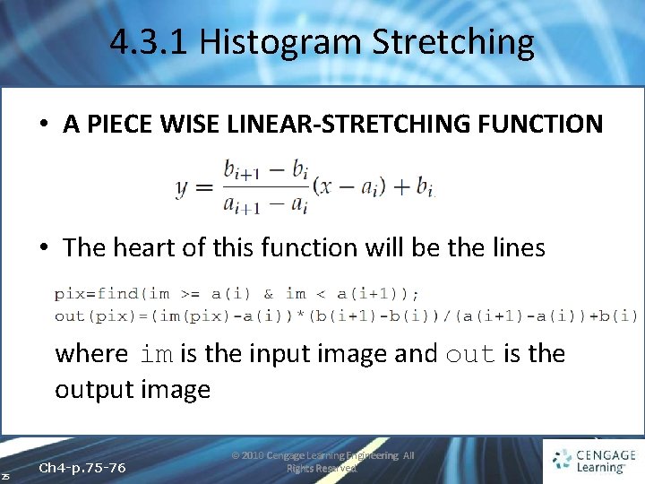
4. 3. 1 Histogram Stretching • A PIECE WISE LINEAR-STRETCHING FUNCTION • The heart of this function will be the lines where im is the input image and out is the output image 25 Ch 4 -p. 75 -76 © 2010 Cengage Learning Engineering. All Rights Reserved.
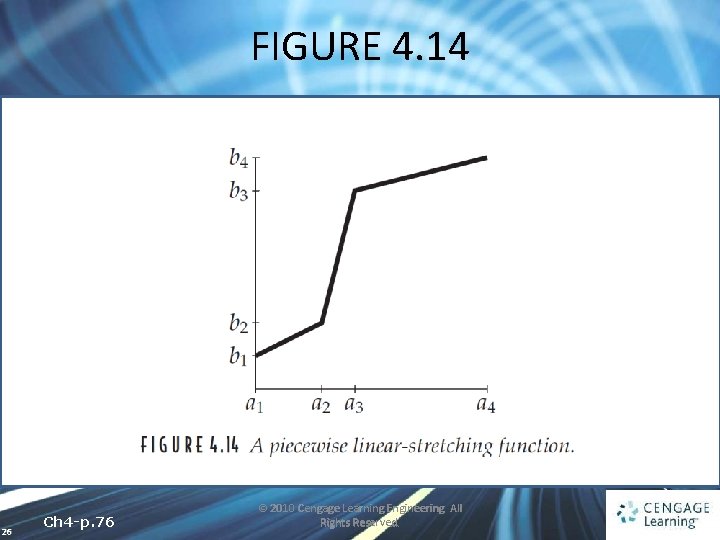
FIGURE 4. 14 26 Ch 4 -p. 76 © 2010 Cengage Learning Engineering. All Rights Reserved.
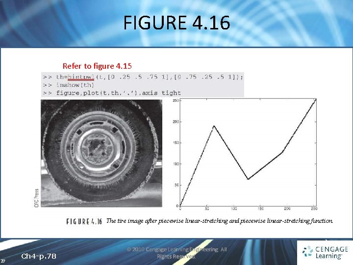
FIGURE 4. 16 Refer to figure 4. 15 The tire image after piecewise linear-stretching and piecewise linear-stretching function. 27 Ch 4 -p. 78 © 2010 Cengage Learning Engineering. All Rights Reserved.
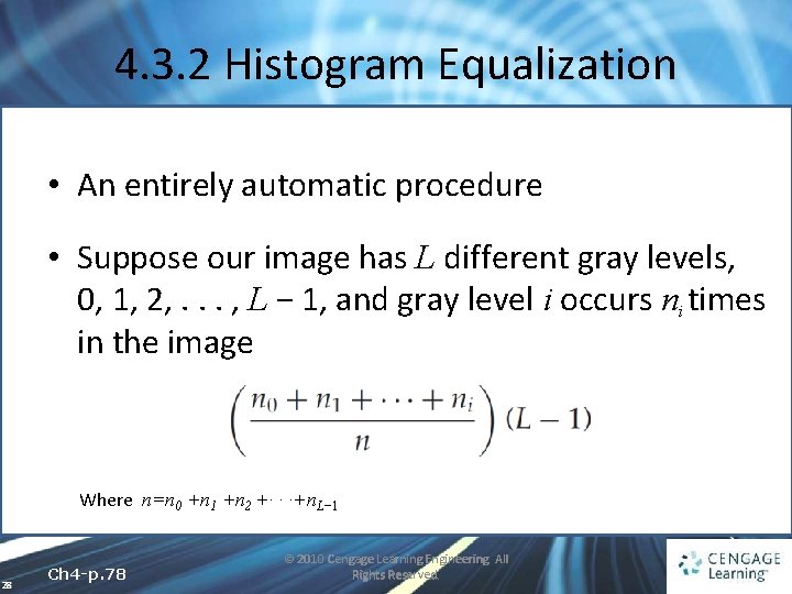
4. 3. 2 Histogram Equalization • An entirely automatic procedure • Suppose our image has L different gray levels, 0, 1, 2, . . . , L − 1, and gray level i occurs ni times in the image Where n=n 0 +n 1 +n 2 +· · ·+n. L− 1 28 Ch 4 -p. 78 © 2010 Cengage Learning Engineering. All Rights Reserved.
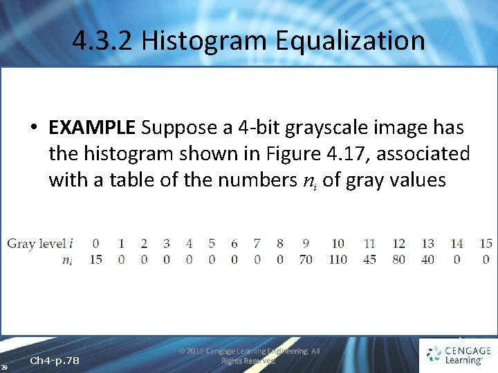
4. 3. 2 Histogram Equalization • EXAMPLE Suppose a 4 -bit grayscale image has the histogram shown in Figure 4. 17, associated with a table of the numbers ni of gray values 29 Ch 4 -p. 78 © 2010 Cengage Learning Engineering. All Rights Reserved.
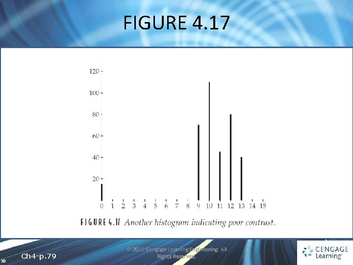
FIGURE 4. 17 30 Ch 4 -p. 79 © 2010 Cengage Learning Engineering. All Rights Reserved.
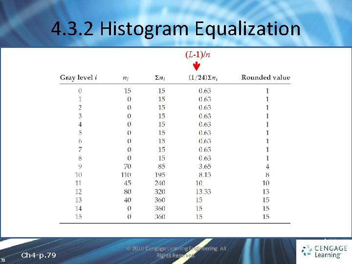
4. 3. 2 Histogram Equalization (L-1)/n 31 Ch 4 -p. 79 © 2010 Cengage Learning Engineering. All Rights Reserved.
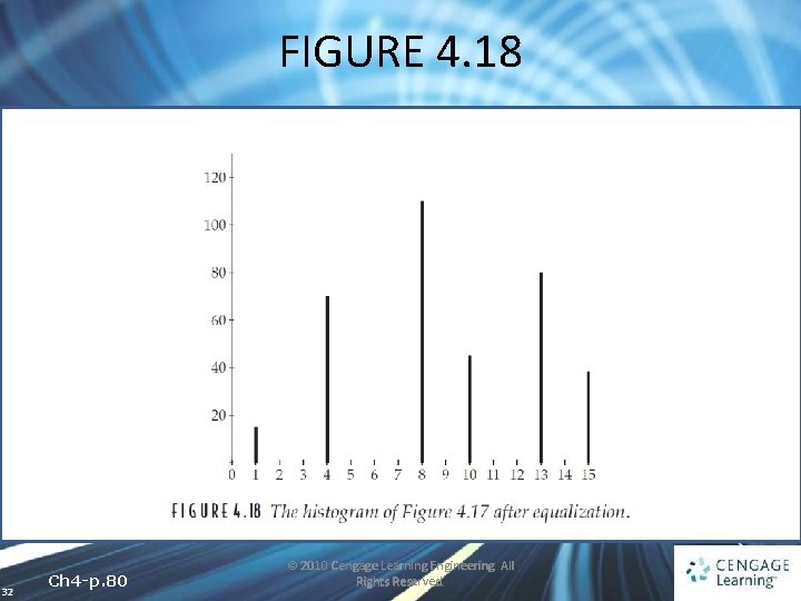
FIGURE 4. 18 32 Ch 4 -p. 80 © 2010 Cengage Learning Engineering. All Rights Reserved.
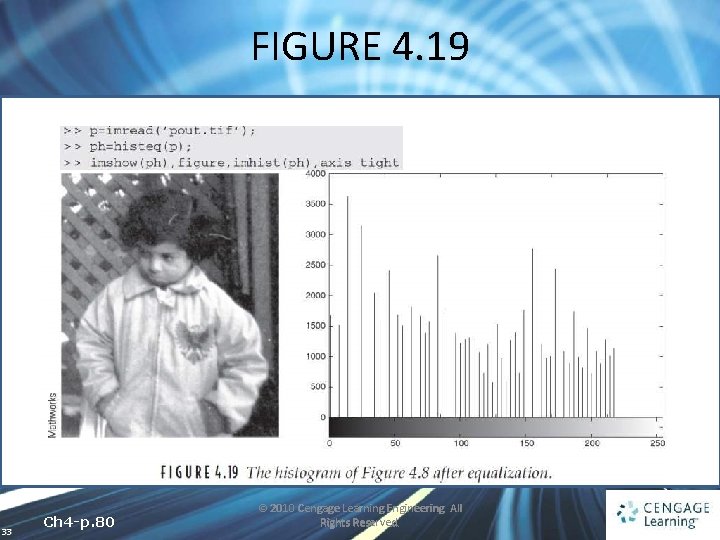
FIGURE 4. 19 33 Ch 4 -p. 80 © 2010 Cengage Learning Engineering. All Rights Reserved.
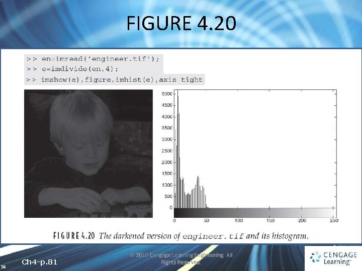
FIGURE 4. 20 34 Ch 4 -p. 81 © 2010 Cengage Learning Engineering. All Rights Reserved.
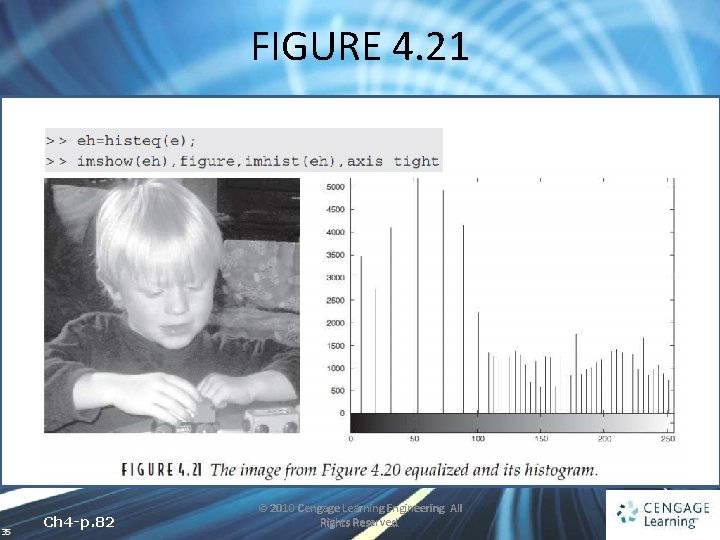
FIGURE 4. 21 35 Ch 4 -p. 82 © 2010 Cengage Learning Engineering. All Rights Reserved.
4. 3. 2 Histogram Equalization • WHY IT WORKS If we were to treat the image as a continuous function f (x, y) and the histogram as the area between different contours, then we can treat the histogram as a probability density function. 36 Ch 4 -p. 82 -83 © 2010 Cengage Learning Engineering. All Rights Reserved.
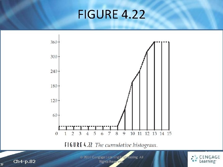
FIGURE 4. 22 37 Ch 4 -p. 82 © 2010 Cengage Learning Engineering. All Rights Reserved.
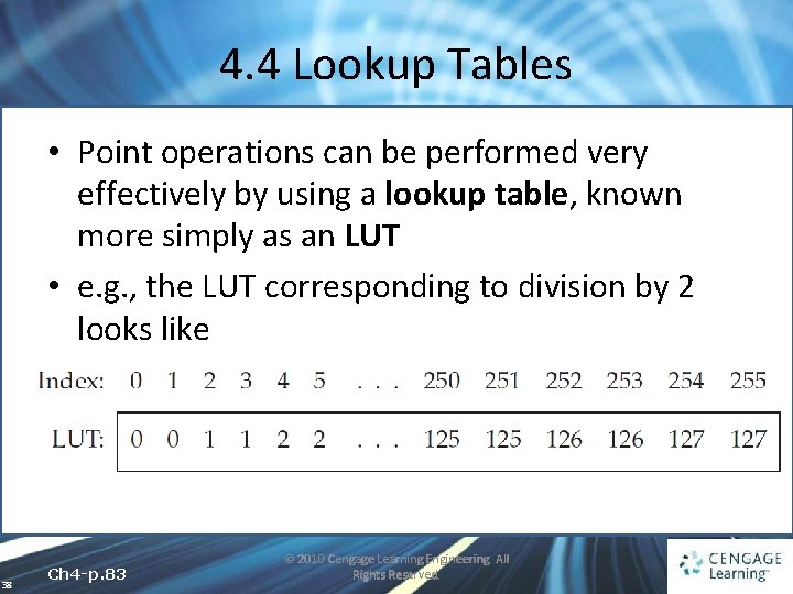
4. 4 Lookup Tables • Point operations can be performed very effectively by using a lookup table, known more simply as an LUT • e. g. , the LUT corresponding to division by 2 looks like 38 Ch 4 -p. 83 © 2010 Cengage Learning Engineering. All Rights Reserved.
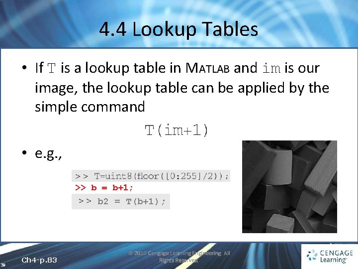
4. 4 Lookup Tables • If T is a lookup table in MATLAB and im is our image, the lookup table can be applied by the simple command • e. g. , >> b = b+1; >> 39 Ch 4 -p. 83 b 2 = T(b+1); © 2010 Cengage Learning Engineering. All Rights Reserved.
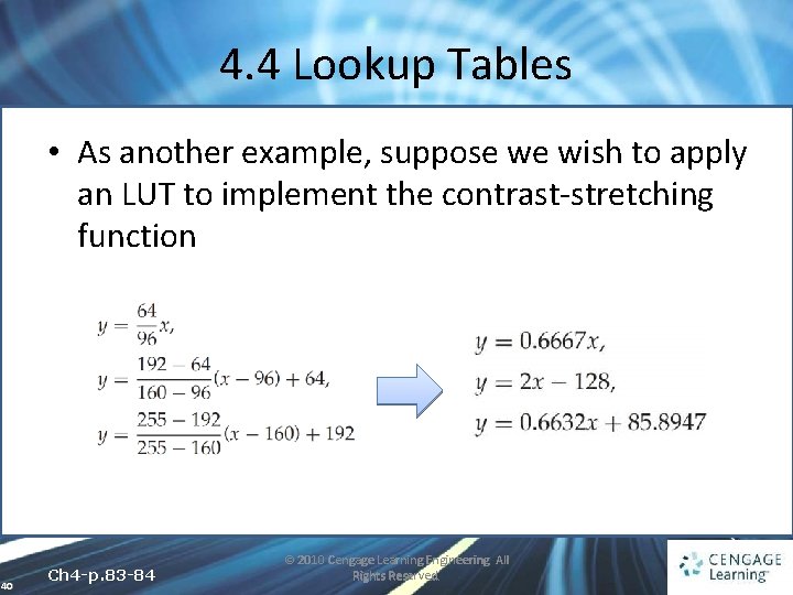
4. 4 Lookup Tables • As another example, suppose we wish to apply an LUT to implement the contrast-stretching function 40 Ch 4 -p. 83 -84 © 2010 Cengage Learning Engineering. All Rights Reserved.
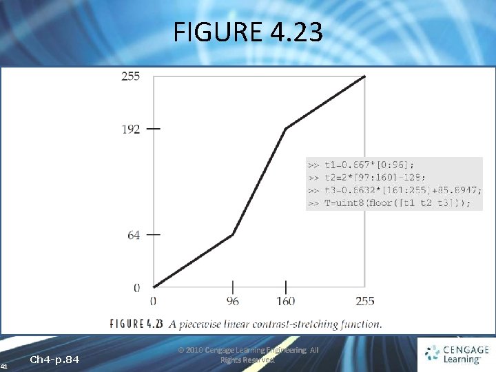
FIGURE 4. 23 41 Ch 4 -p. 84 © 2010 Cengage Learning Engineering. All Rights Reserved.
- Slides: 41