Introduction to Digital Image Processing with MATLAB Asia
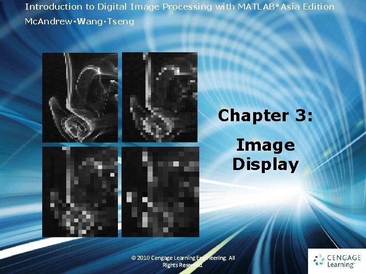
Introduction to Digital Image Processing with MATLAB® Asia Edition Mc. Andrew‧Wang‧Tseng Chapter 3: Image Display 1 © 2010 Cengage Learning Engineering. All Rights Reserved. 1
3. 1 Introduction • We take a closer look at the use of the imshow function • We look at image quality and how that may be affected by various image attributes • For human vision in general, the preference is for images to be sharp and detailed 2 Ch 3 -p. 41 © 2010 Cengage Learning Engineering. All Rights Reserved.
3. 2 Basics of Image Display • There are many factors that will affect the display ü ambient lighting, ü the monitor type and settings, ü the graphics card, and ü monitor resolution 3 Ch 3 -p. 41 © 2010 Cengage Learning Engineering. All Rights Reserved.
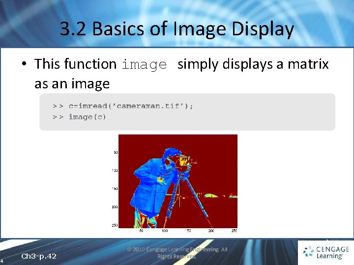
3. 2 Basics of Image Display • This function image simply displays a matrix as an image 4 Ch 3 -p. 42 © 2010 Cengage Learning Engineering. All Rights Reserved.
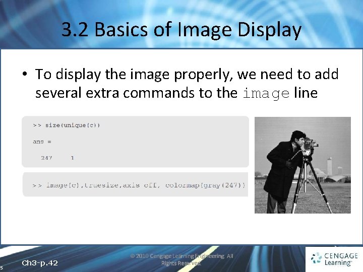
3. 2 Basics of Image Display • To display the image properly, we need to add several extra commands to the image line 5 Ch 3 -p. 42 © 2010 Cengage Learning Engineering. All Rights Reserved.
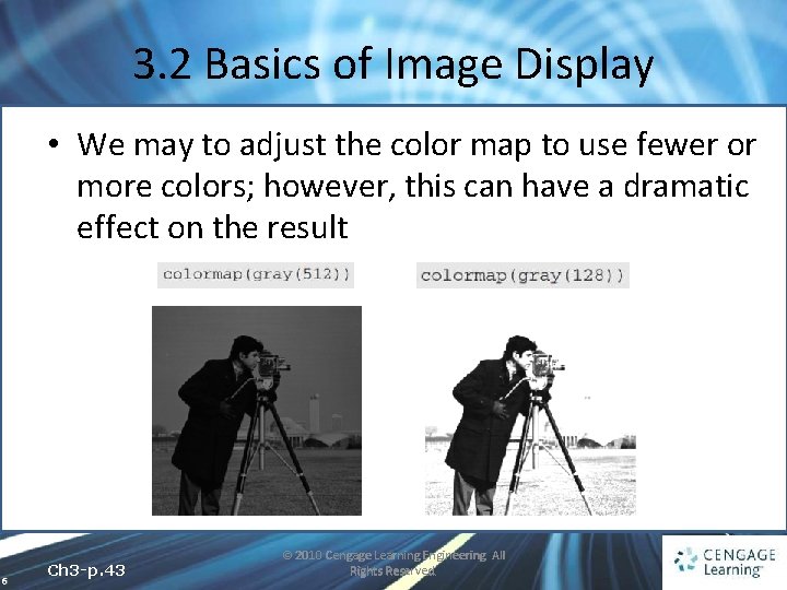
3. 2 Basics of Image Display • We may to adjust the color map to use fewer or more colors; however, this can have a dramatic effect on the result 6 Ch 3 -p. 43 © 2010 Cengage Learning Engineering. All Rights Reserved.
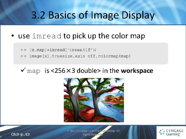
3. 2 Basics of Image Display • use imread to pick up the color map ü map is <256× 3 double> in the workspace 7 Ch 3 -p. 43 © 2010 Cengage Learning Engineering. All Rights Reserved.
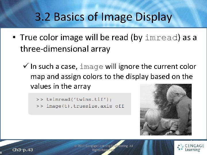
3. 2 Basics of Image Display • True color image will be read (by imread) as a three-dimensional array ü In such a case, image will ignore the current color map and assign colors to the display based on the values in the array 8 Ch 3 -p. 43 © 2010 Cengage Learning Engineering. All Rights Reserved.
3. 3 The imshow Function • We have two choices with a matrix of type double: ü Convert to type uint 8 and then display ü Display the matrix directly • imshow will display a matrix of type double as a grayscale image (matrix elements are between 0 and 1) 9 Ch 3 -p. 44 © 2010 Cengage Learning Engineering. All Rights Reserved.
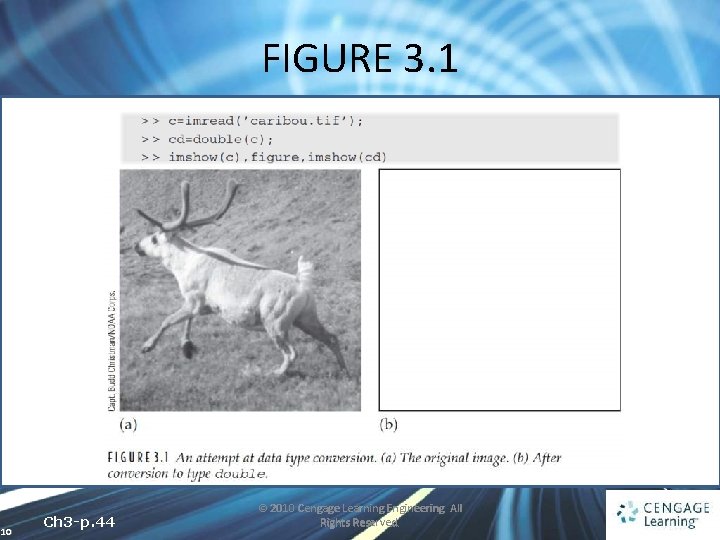
FIGURE 3. 1 10 Ch 3 -p. 44 © 2010 Cengage Learning Engineering. All Rights Reserved.
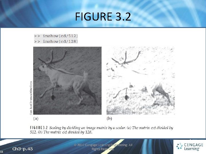
FIGURE 3. 2 11 Ch 3 -p. 45 © 2010 Cengage Learning Engineering. All Rights Reserved.
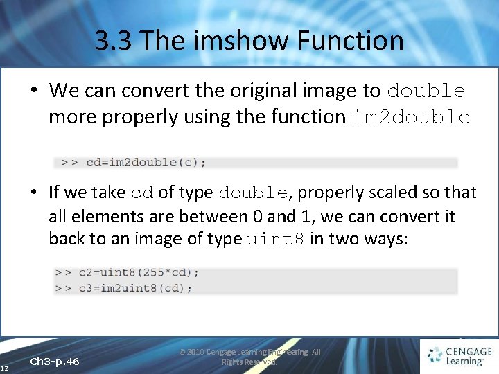
3. 3 The imshow Function • We can convert the original image to double more properly using the function im 2 double • If we take cd of type double, properly scaled so that all elements are between 0 and 1, we can convert it back to an image of type uint 8 in two ways: 12 Ch 3 -p. 46 © 2010 Cengage Learning Engineering. All Rights Reserved.
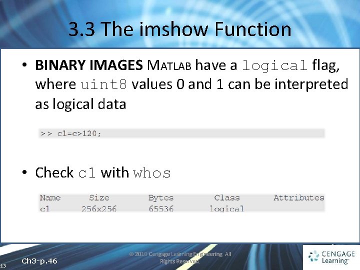
3. 3 The imshow Function • BINARY IMAGES MATLAB have a logical flag, where uint 8 values 0 and 1 can be interpreted as logical data • Check c 1 with whos 13 Ch 3 -p. 46 © 2010 Cengage Learning Engineering. All Rights Reserved.
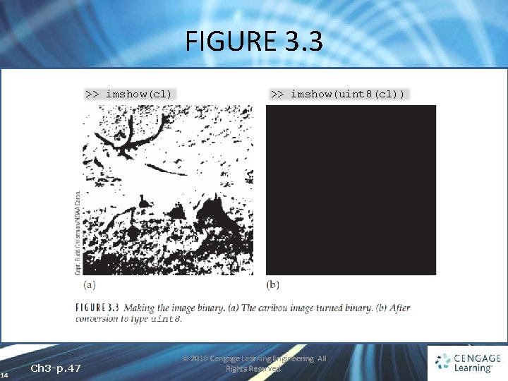
FIGURE 3. 3 >> imshow(cl) 14 Ch 3 -p. 47 >> imshow(uint 8(cl)) © 2010 Cengage Learning Engineering. All Rights Reserved.
3. 4 Bit Planes • Grayscale images can be transformed into a sequence of binary images by breaking them up into their bitplanes • The zeroth bit plane ü the least significant bit plane • The seventh bit plane ü the most significant bit plane 15 Ch 3 -p. 48 © 2010 Cengage Learning Engineering. All Rights Reserved.
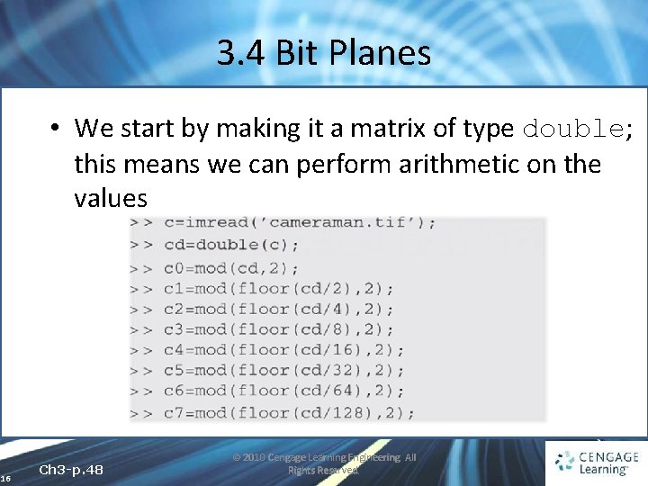
3. 4 Bit Planes • We start by making it a matrix of type double; this means we can perform arithmetic on the values 16 Ch 3 -p. 48 © 2010 Cengage Learning Engineering. All Rights Reserved.
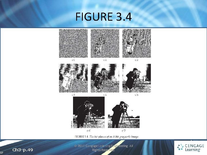
FIGURE 3. 4 17 Ch 3 -p. 49 © 2010 Cengage Learning Engineering. All Rights Reserved.
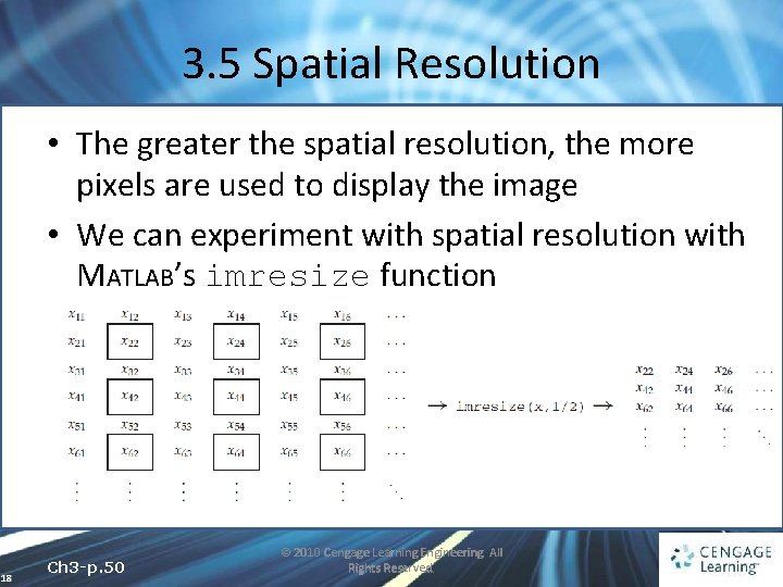
3. 5 Spatial Resolution • The greater the spatial resolution, the more pixels are used to display the image • We can experiment with spatial resolution with MATLAB’s imresize function 18 Ch 3 -p. 50 © 2010 Cengage Learning Engineering. All Rights Reserved.
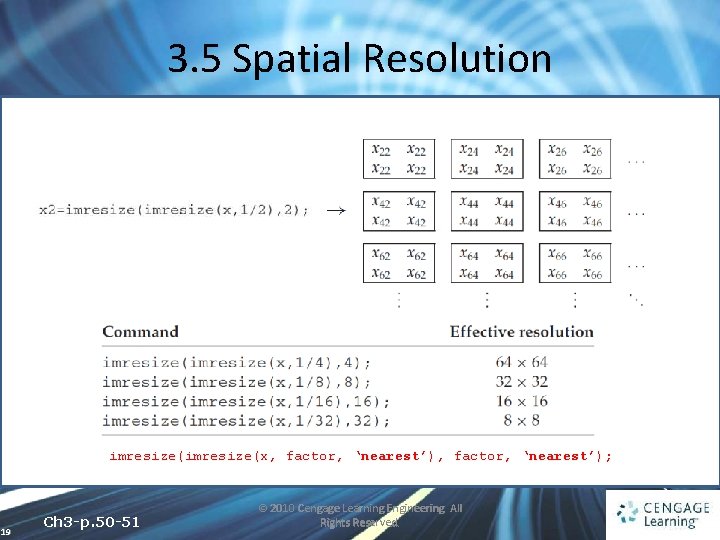
3. 5 Spatial Resolution imresize(x, factor, ‘nearest’); 19 Ch 3 -p. 50 -51 © 2010 Cengage Learning Engineering. All Rights Reserved.
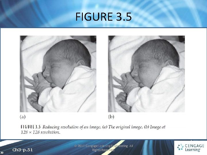
FIGURE 3. 5 20 Ch 3 -p. 51 © 2010 Cengage Learning Engineering. All Rights Reserved.
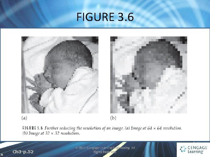
FIGURE 3. 6 21 Ch 3 -p. 52 © 2010 Cengage Learning Engineering. All Rights Reserved.
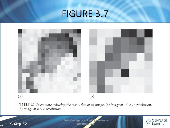
FIGURE 3. 7 22 Ch 3 -p. 52 © 2010 Cengage Learning Engineering. All Rights Reserved.
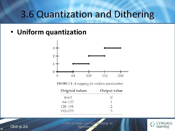
3. 6 Quantization and Dithering • Uniform quantization 23 Ch 3 -p. 52 © 2010 Cengage Learning Engineering. All Rights Reserved.
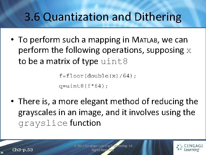
3. 6 Quantization and Dithering • To perform such a mapping in MATLAB, we can perform the following operations, supposing x to be a matrix of type uint 8 • There is, a more elegant method of reducing the grayscales in an image, and it involves using the grayslice function 24 Ch 3 -p. 53 © 2010 Cengage Learning Engineering. All Rights Reserved.
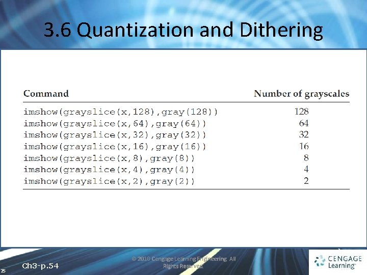
3. 6 Quantization and Dithering 25 Ch 3 -p. 54 © 2010 Cengage Learning Engineering. All Rights Reserved.
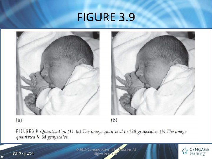
FIGURE 3. 9 26 Ch 3 -p. 54 © 2010 Cengage Learning Engineering. All Rights Reserved.

FIGURE 3. 10 27 Ch 3 -p. 55 © 2010 Cengage Learning Engineering. All Rights Reserved.
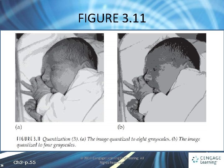
FIGURE 3. 11 28 Ch 3 -p. 55 © 2010 Cengage Learning Engineering. All Rights Reserved.
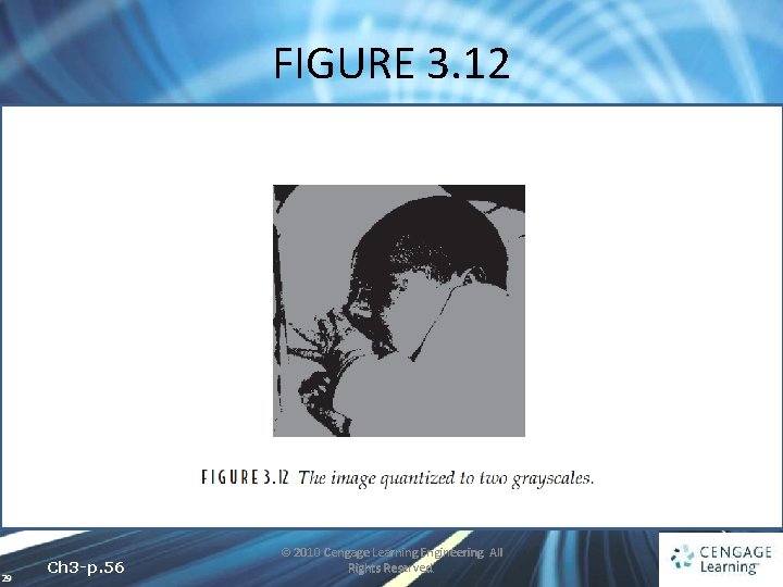
FIGURE 3. 12 29 Ch 3 -p. 56 © 2010 Cengage Learning Engineering. All Rights Reserved.
3. 6 Quantization and Dithering • DITHERING In general terms, refers to the process of reducing the number of colors in an image • Representing an image with only two tones is also known as halftoning 30 Ch 3 -p. 56 © 2010 Cengage Learning Engineering. All Rights Reserved.
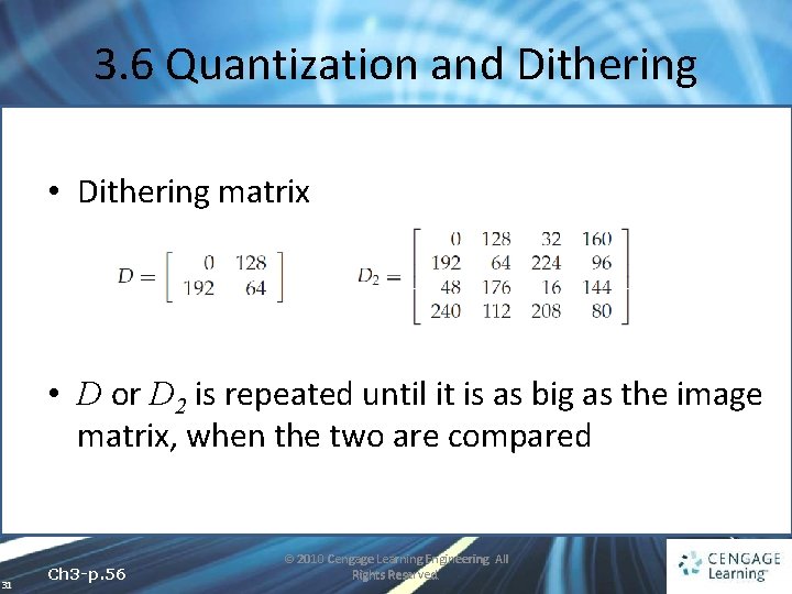
3. 6 Quantization and Dithering • Dithering matrix • D or D 2 is repeated until it is as big as the image matrix, when the two are compared 31 Ch 3 -p. 56 © 2010 Cengage Learning Engineering. All Rights Reserved.
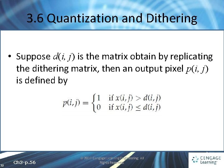
3. 6 Quantization and Dithering • Suppose d(i, j) is the matrix obtain by replicating the dithering matrix, then an output pixel p(i, j) is defined by 32 Ch 3 -p. 56 © 2010 Cengage Learning Engineering. All Rights Reserved.
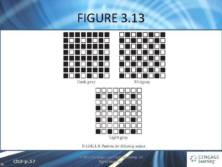
FIGURE 3. 13 33 Ch 3 -p. 57 © 2010 Cengage Learning Engineering. All Rights Reserved.
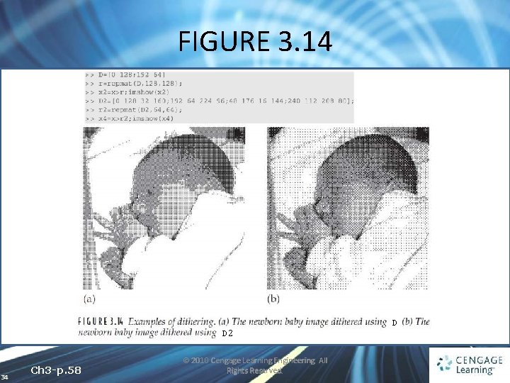
FIGURE 3. 14 D 2 34 Ch 3 -p. 58 © 2010 Cengage Learning Engineering. All Rights Reserved. D
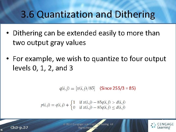
3. 6 Quantization and Dithering • Dithering can be extended easily to more than two output gray values • For example, we wish to quantize to four output levels 0, 1, 2, and 3 (Since 255/3 = 85) 35 Ch 3 -p. 57 © 2010 Cengage Learning Engineering. All Rights Reserved.
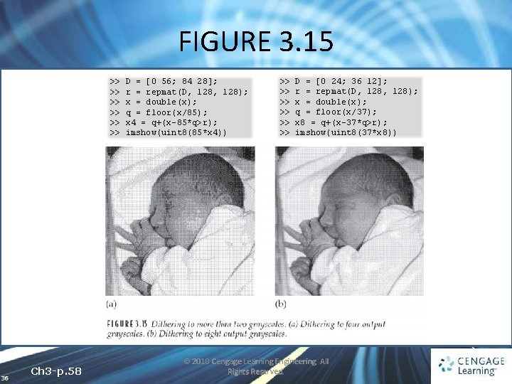
FIGURE 3. 15 >> >> >> 36 Ch 3 -p. 58 D = [0 56; 84 28]; r = repmat(D, 128); x = double(x); q = floor(x/85); x 4 = q+(x-85*q>r); imshow(uint 8(85*x 4)) >> >> >> D = [0 24; 36 12]; r = repmat(D, 128); x = double(x); q = floor(x/37); x 8 = q+(x-37*q>r); imshow(uint 8(37*x 8)) © 2010 Cengage Learning Engineering. All Rights Reserved.
3. 6 Quantization and Dithering • ERROR DIFFUSION ü The image is quantized at two levels ü For each pixel we take into account the error between its gray value and its quantized value ü The idea is to spread this error over neighboring pixels 37 Ch 3 -p. 59 © 2010 Cengage Learning Engineering. All Rights Reserved.
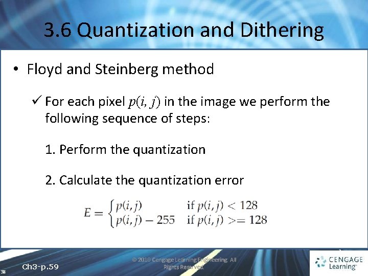
3. 6 Quantization and Dithering • Floyd and Steinberg method ü For each pixel p(i, j) in the image we perform the following sequence of steps: 1. Perform the quantization 2. Calculate the quantization error 38 Ch 3 -p. 59 © 2010 Cengage Learning Engineering. All Rights Reserved.
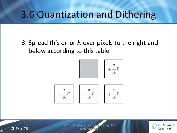
3. 6 Quantization and Dithering 3. Spread this error E over pixels to the right and below according to this table 39 Ch 3 -p. 59 © 2010 Cengage Learning Engineering. All Rights Reserved.
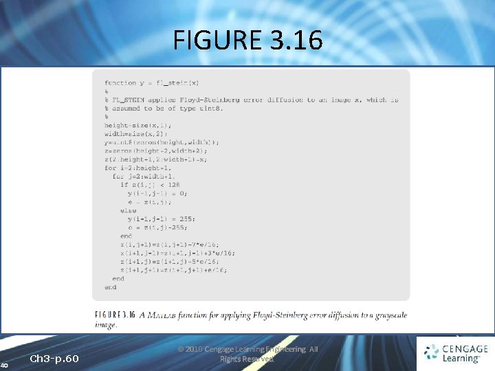
FIGURE 3. 16 40 Ch 3 -p. 60 © 2010 Cengage Learning Engineering. All Rights Reserved.
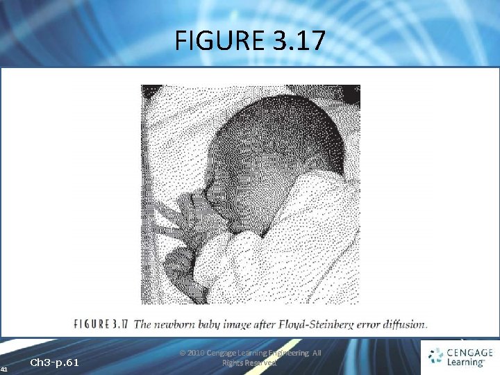
FIGURE 3. 17 41 Ch 3 -p. 61 © 2010 Cengage Learning Engineering. All Rights Reserved.
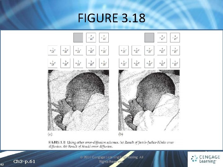
FIGURE 3. 18 42 Ch 3 -p. 61 © 2010 Cengage Learning Engineering. All Rights Reserved.
- Slides: 42