Introduction to Digital Image Analysis Kurt Thorn NIC

Introduction to Digital Image Analysis Kurt Thorn NIC

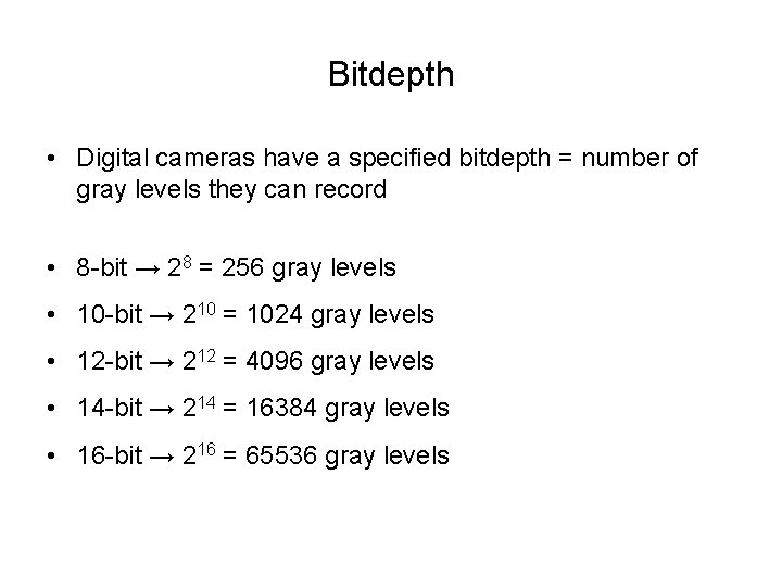
Bitdepth • Digital cameras have a specified bitdepth = number of gray levels they can record • 8 -bit → 28 = 256 gray levels • 10 -bit → 210 = 1024 gray levels • 12 -bit → 212 = 4096 gray levels • 14 -bit → 214 = 16384 gray levels • 16 -bit → 216 = 65536 gray levels

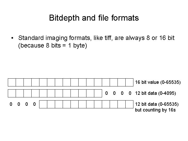
Bitdepth and file formats • Standard imaging formats, like tiff, are always 8 or 16 bit (because 8 bits = 1 byte) 16 bit value (0 -65535) 0 0 0 0 12 bit data (0 -4095) 12 bit data (0 -65535) but counting by 16 s

Color Images • Color images are made up of three gray scale images, one for each of red, green, and blue • Can be 8 or 16 bits per channel

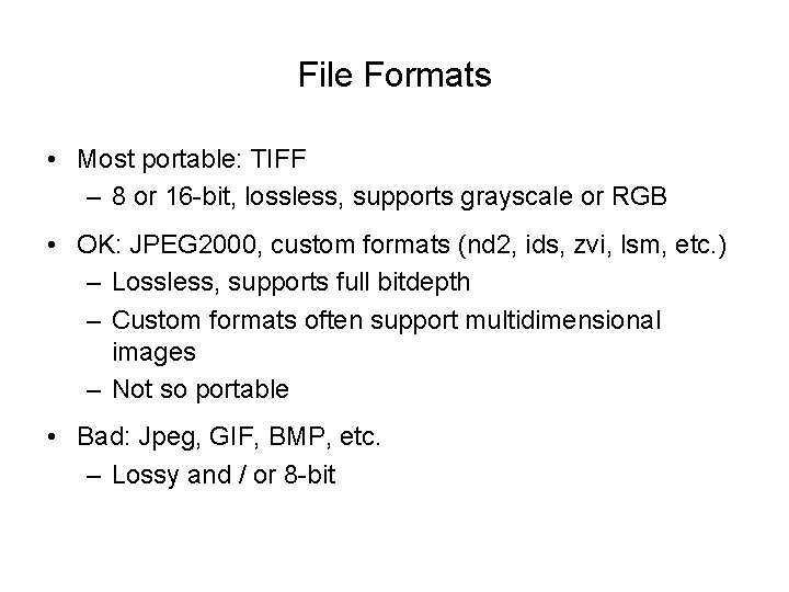
File Formats • Most portable: TIFF – 8 or 16 -bit, lossless, supports grayscale or RGB • OK: JPEG 2000, custom formats (nd 2, ids, zvi, lsm, etc. ) – Lossless, supports full bitdepth – Custom formats often support multidimensional images – Not so portable • Bad: Jpeg, GIF, BMP, etc. – Lossy and / or 8 -bit

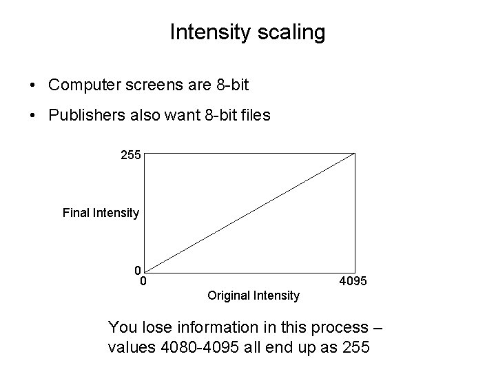
Intensity scaling • Computer screens are 8 -bit • Publishers also want 8 -bit files 255 Final Intensity 0 0 4095 Original Intensity You lose information in this process – values 4080 -4095 all end up as 255

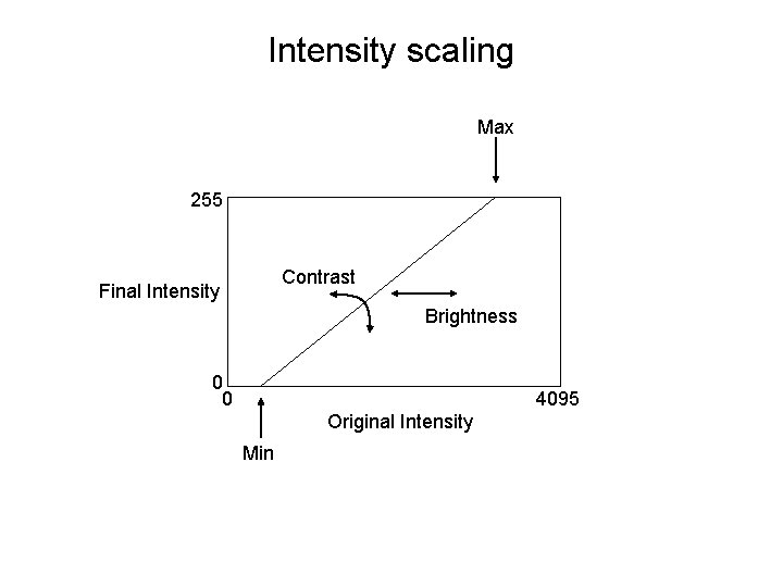
Intensity scaling Max 255 Contrast Final Intensity Brightness 0 0 4095 Original Intensity Min

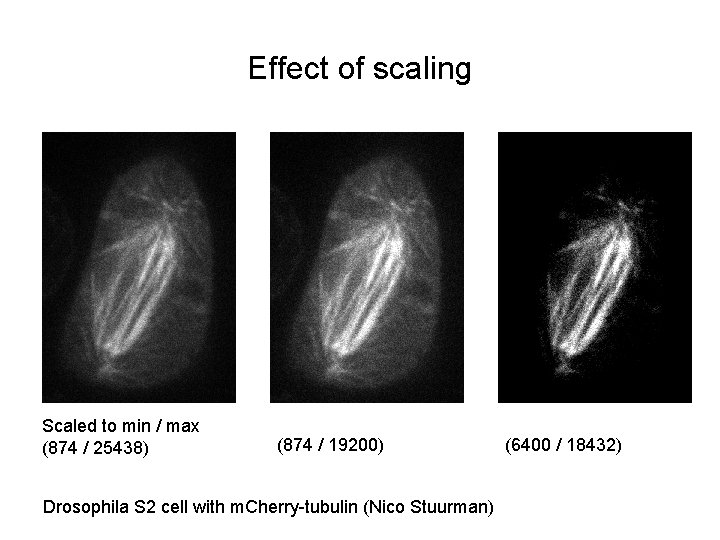
Effect of scaling Scaled to min / max (874 / 25438) (874 / 19200) Drosophila S 2 cell with m. Cherry-tubulin (Nico Stuurman) (6400 / 18432)

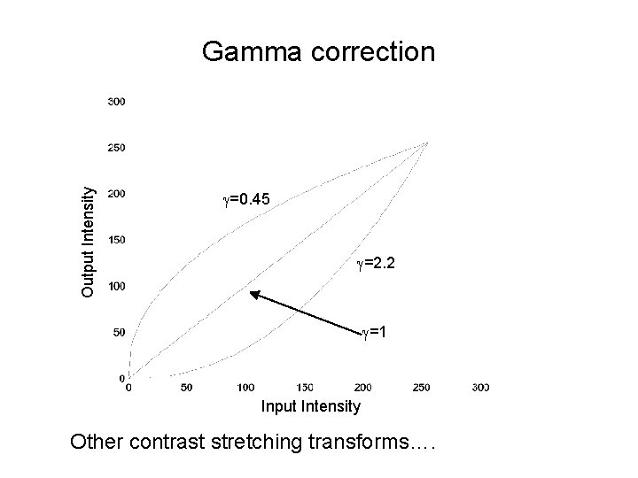
Output Intensity Gamma correction g=0. 45 g=2. 2 g=1 Input Intensity Other contrast stretching transforms….

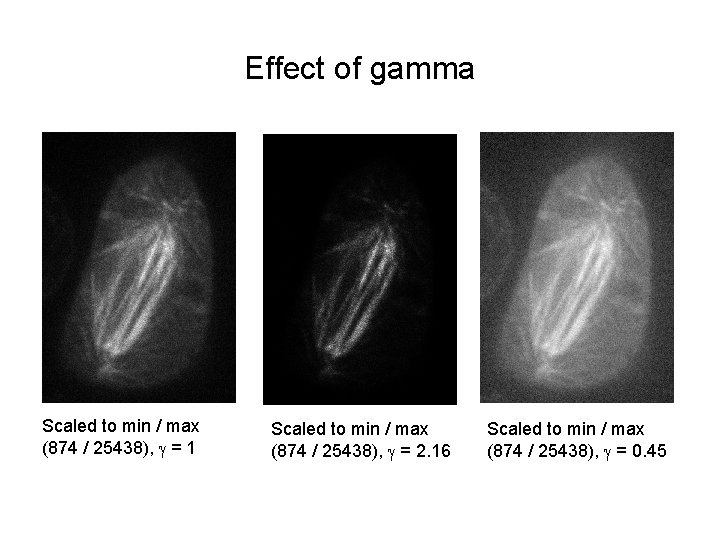
Effect of gamma Scaled to min / max (874 / 25438), g = 1 Scaled to min / max (874 / 25438), g = 2. 16 Scaled to min / max (874 / 25438), g = 0. 45

What are acceptable image manipulations? • JCB has the best guidelines – http: //jcb. rupress. org/misc/ifora. shtml#image_aquisition – http: //jcb. rupress. org/cgi/content/full/166/1/1 • Brightness and contrast adjustments ok, so long as done over whole image and don’t obscure or eliminate background • Nonlinear adjustments (like gamma) must be disclosed • No cutting and pasting of regions within an image (e. g. individual cells)

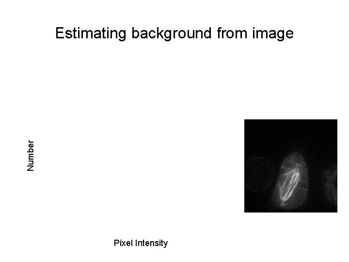
Background correction • Cameras have a non-zero offset • There can also be background fluorescence due to media autofluorescence, etc. • Want to correct for this by background subtraction – Camera dark image – Estimate background from image

Number Estimating background from image Pixel Intensity

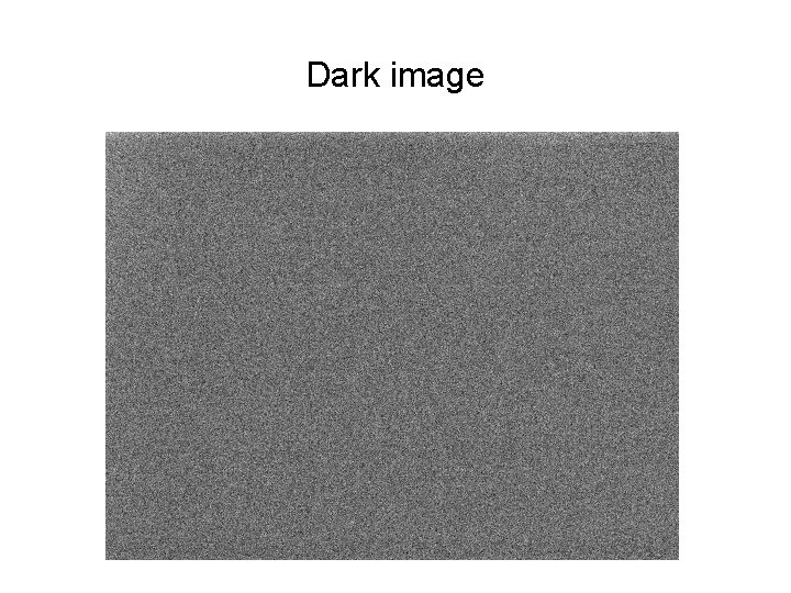
Dark image • Acquired with no light going to the camera – Allows you to measure instrument background – Can detect what’s real background autofluorescence

Dark image

Shading correction • Measure and correct for nonuniformity in illumination and detection • Image a uniform fluorescent sample

Shading correction

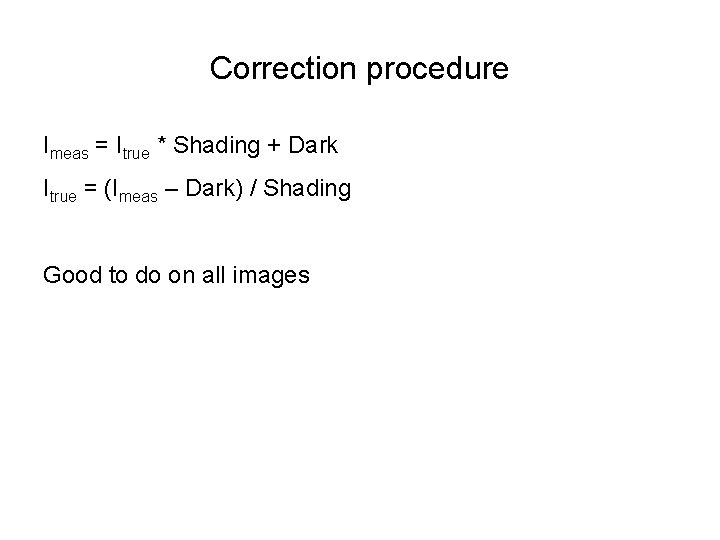
Correction procedure Imeas = Itrue * Shading + Dark Itrue = (Imeas – Dark) / Shading Good to do on all images

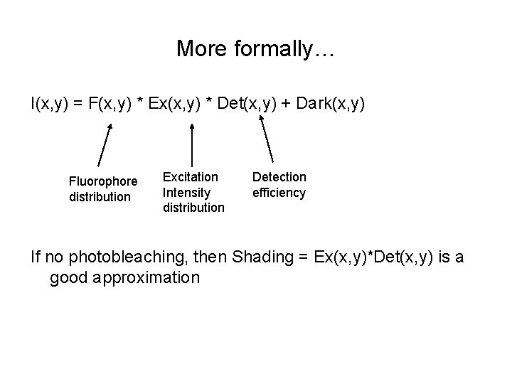
More formally… I(x, y) = F(x, y) * Ex(x, y) * Det(x, y) + Dark(x, y) Fluorophore distribution Excitation Intensity distribution Detection efficiency If no photobleaching, then Shading = Ex(x, y)*Det(x, y) is a good approximation

If photobleaching… I(x, y) = (F(x, y) / k*Ex(x, y)) * [1 -exp(-k*Ex(x, y)*t)] * Det(x, y) + Dark(x, y) Yuck If you have significant photobleaching and significant excitation non-uniformity, shading correction breaks down Can actually lead to contrast inversion (!)

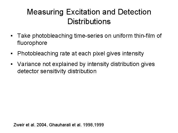
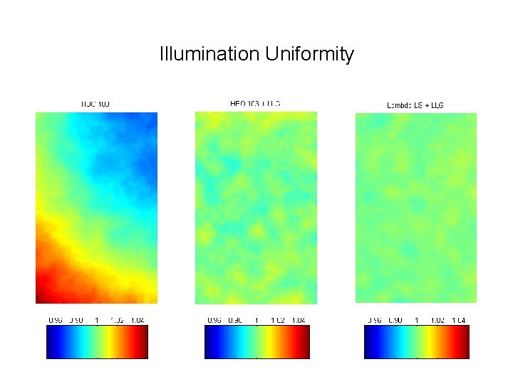
Measuring Excitation and Detection Distributions • Take photobleaching time-series on uniform thin-film of fluorophore • Photobleaching rate at each pixel gives intensity • Variance not explained by intensity distribution gives detector sensitivity distribution Zweir et al. 2004, Ghauharali et al. 1998, 1999

Illumination Uniformity

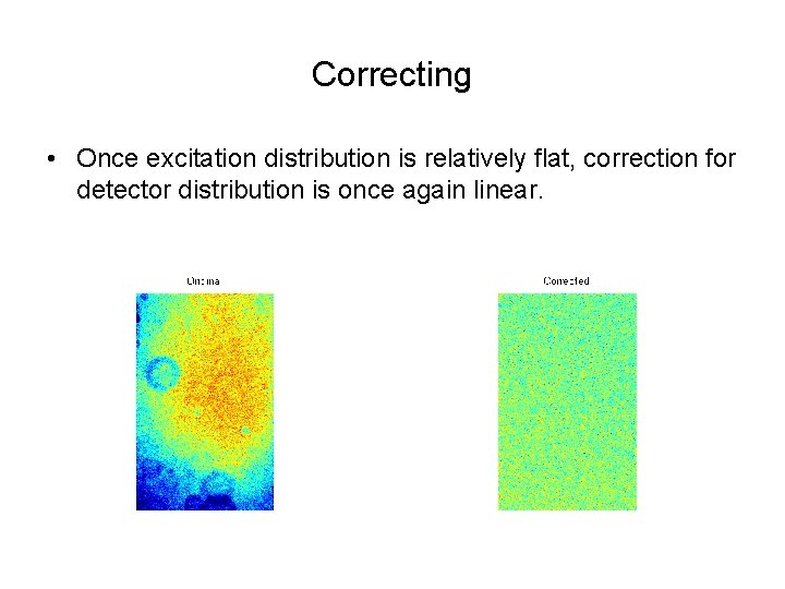
Correcting • Once excitation distribution is relatively flat, correction for detector distribution is once again linear.

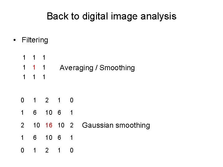
Back to digital image analysis • Filtering 1 1 1 1 1 0 1 2 1 0 1 6 10 6 1 2 10 16 10 2 1 6 10 6 1 0 1 2 0 Averaging / Smoothing 1 Gaussian smoothing

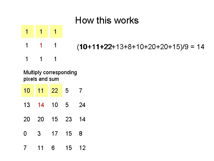
How this works 1 1 1 1 1 (10+11+22+13+8+10+20+20+15)/9 10 +11+22 = 14 Multiply corresponding pixels and sum 10 11 22 5 7 13 814 10 5 24 20 20 15 23 14 0 3 17 15 8 7 11 6 15 12

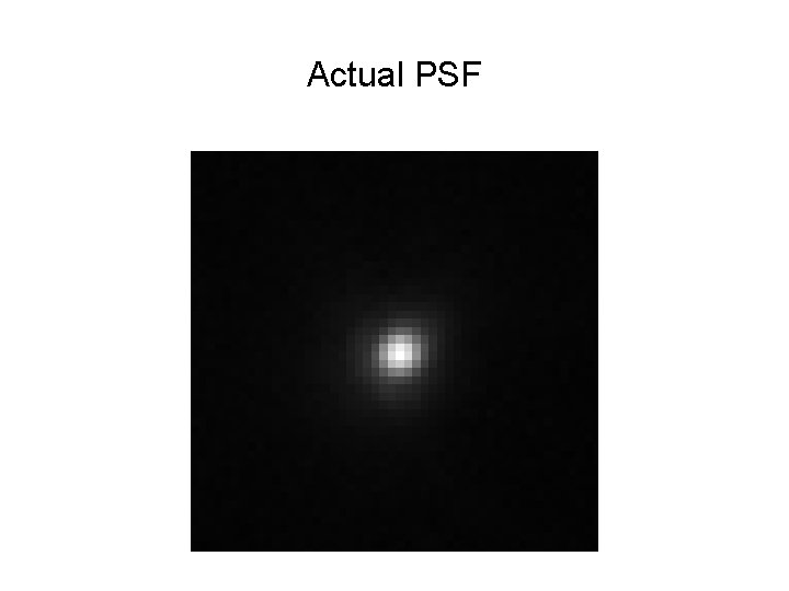
Why smooth? • If your image is sampled appropriately (at Nyquist) the point spread function will be spread out over multiple pixels • Properly exploiting this redundancy requires deconvolution • But smoothing helps • Also reduces single pixel noise artifacts that can’t be real

Actual PSF

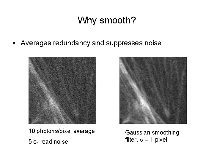
Why smooth? • Averages redundancy and suppresses noise 10 photons/pixel average 5 e- read noise Gaussian smoothing filter, s = 1 pixel

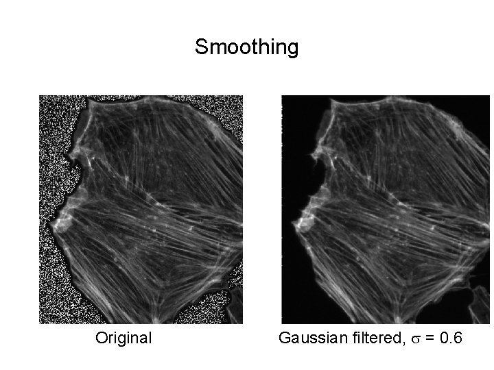
Smoothing Original Gaussian filtered, s = 0. 6

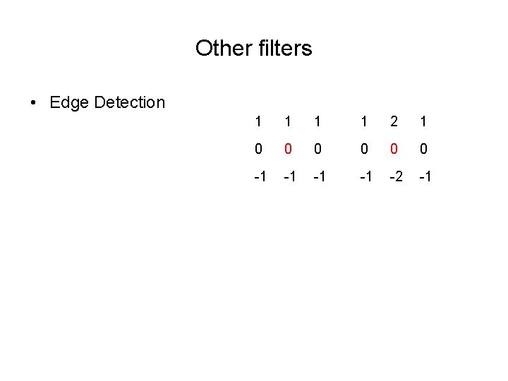
Other filters • Edge Detection 1 1 2 1 0 0 0 -1 -1 -2 -1

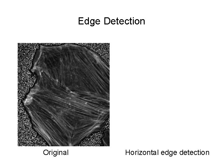
Edge Detection Original Horizontal edge detection

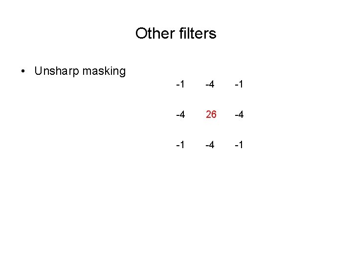
Other filters • Unsharp masking -1 -4 26 -4 -1

Unsharp Masking Original Unsharp masked

Nonlinear filters • Can do things like median filtering – replace center pixel by median value within box • Good for smoothing while maintaining edges

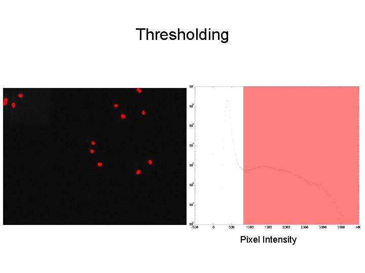
Thresholding Pixel Intensity

One problem with this approach… • It’s biased towards brighter objects • Ideally would use second channel to independently define objects to measure

Binary images • Thresholding gives you a binary image; 1 inside an object, 0 elsewhere • This can be used to identify objects • It can also be manipulated

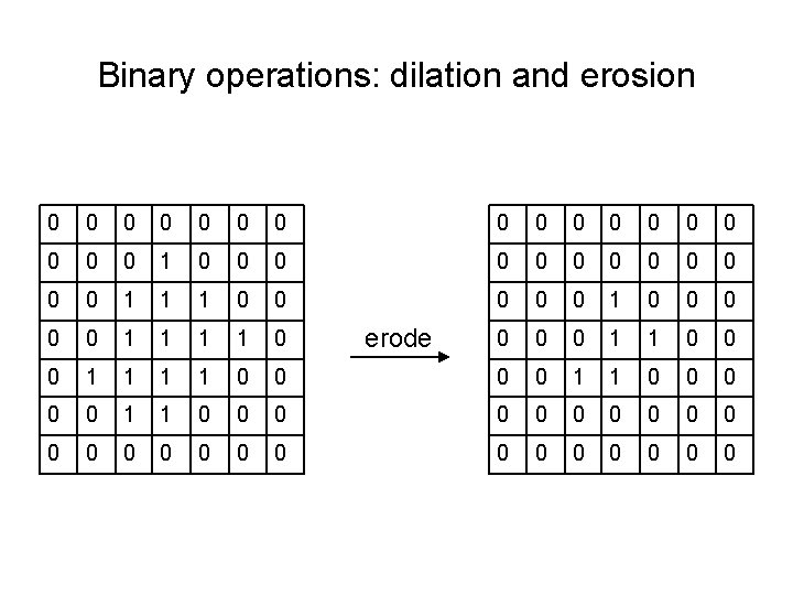
Binary operations: dilation and erosion 0 0 0 0 0 1 0 0 0 1 1 1 0 0 0 0 0 1 1 1 1 0 0 0 0 0 1 1 0 0 0 0 0 0 erode

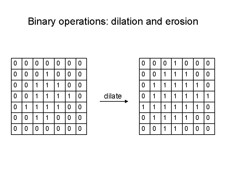
Binary operations: dilation and erosion 0 0 0 0 0 1 0 0 0 1 1 1 0 0 0 1 1 1 0 1 1 0 0 1 1 1 0 0 0 1 1 0 0 0 1 1 0 0 0 dilate

Other binary operations • Sequential erosion and dilation – tends to smooth objects • Hole filling • Removing objects at borders

Further reading • Lectures available online: nic. ucsf. edu/edu. html • Gonzalez, Woods, and Eddins: Digital Image Processing (Using Matlab) • Pawley: Handbook of Biological Confocal Microscopy