Introduction to Deep Learning TEI of Crete MSc

Introduction to Deep Learning TEI of Crete - MSc in Informatics and Multimedia Konstantinos Karampidis , MSc

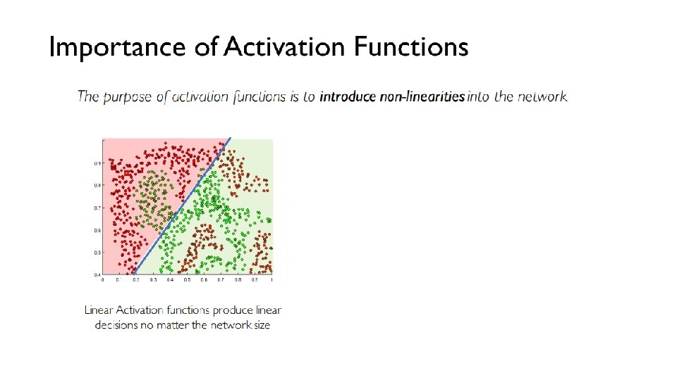
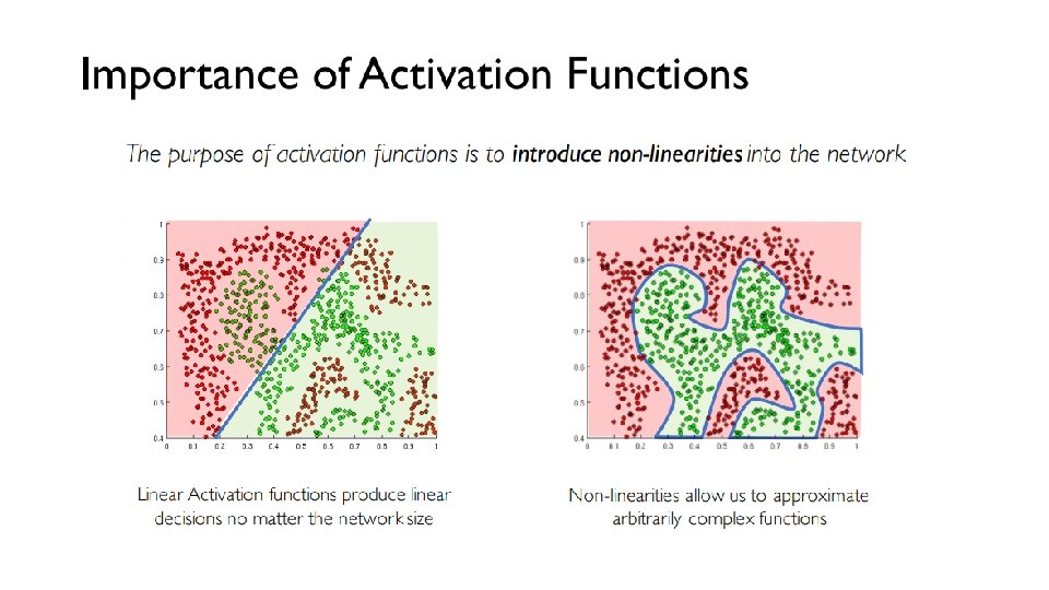
Introduction Deep Learning is a new area of Machine Learning research, which has been introduced with the objective of moving Machine Learning closer to one of its original goals Deep Learning is about learning multiple levels of representation and abstraction that help to make sense of data such as images, sound, and text.

Motivations for Deep Architectures The main motivations for studying learning algorithms for deep architectures are the following: ØInsufficient depth can hurt ØThe brain has a deep architecture ØCognitive processes seem deep

Motivations for Deep Architectures Why Deep Learning? ØInsufficient depth can hurt • With shallow architecture (SVM, NB, KNN, etc. ), the required number of nodes in the graph (i. e. computations, and also number of parameters, when we try to learn the function) may grow very large. • Many functions that can be represented efficiently with a deep architecture cannot be represented efficiently with a shallow one.

Motivations for Deep Architectures Why Deep Learning? ØThe brain has a deep architecture • The visual cortex shows a sequence of areas each of which contains a representation of the input, and signals flow from one to the next. • Note that representations in the brain are in between dense distributed and purely local: they are sparse: about 1% of neurons are active simultaneously in the brain.

Motivations for Deep Architectures Why Deep Learning? Ø Cognitive processes seem deep • Humans organize their ideas and concepts hierarchically. • Humans first learn simpler concepts and then compose them to represent more abstract ones. • Engineers break-up solutions into multiple levels of abstraction and processing

Why Now ?

Until Now…

Deep Learning = Learning Hierarchical Representations

Deep Learning = Learning Hierarchical Representations

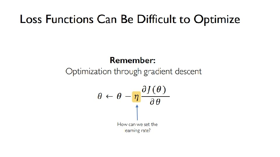
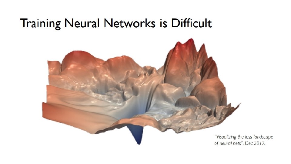
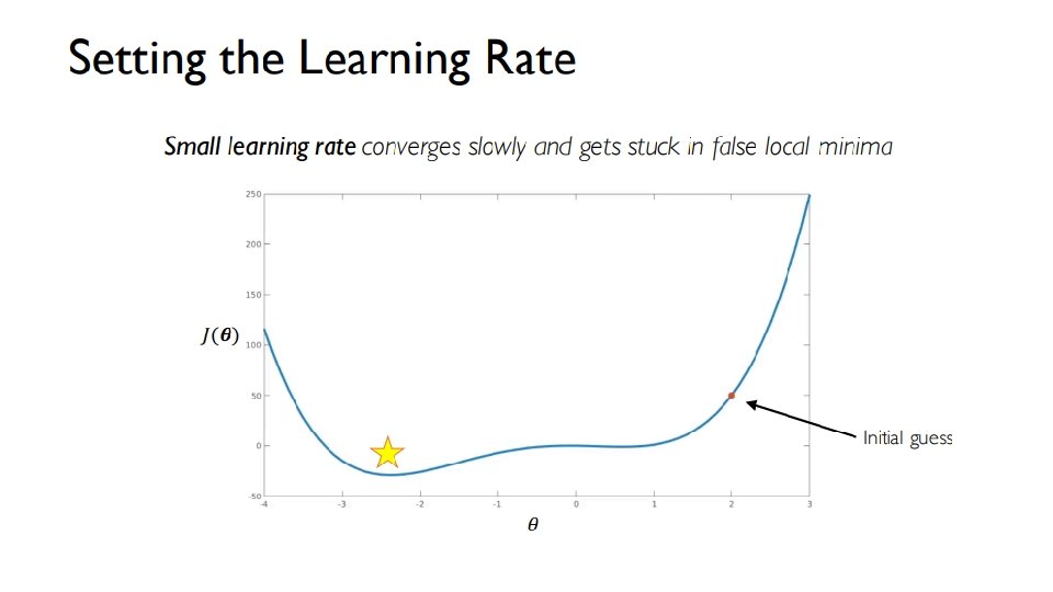
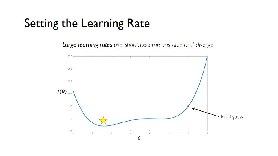
Training Neural Networks

Or

Mini-batches

Conv. Nets ØA supervised deep learning method.

Conv. Nets

Conv. Nets

Conv. Nets

Conv. Nets

Conv. Nets

In CNN terminology, the 3× 3 matrix is called a ‘filter‘ or ‘kernel’ or ‘feature detector’ and the matrix formed by sliding the filter over the image and computing the dot product is called the ‘Convolved Feature’ or ‘Activation Map’ or the ‘Feature Map‘. It is important to note that filters act as feature detectors from the original input image.

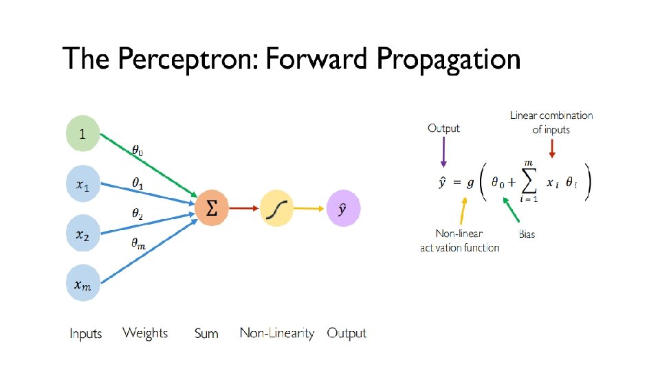
Feature Map Parameters The size of the Feature Map (Convolved Feature) is controlled by three parameters that we need to decide before the convolution step is performed: • Depth: Depth corresponds to the number of filters we use for the convolution operation. In the network shown in Figure, we are performing convolution of the original boat image using three distinct filters, thus producing three different feature maps as shown. You can think of these three feature maps as stacked 2 d matrices, so, the ‘depth’ of the feature map would be three.

Feature Map Parameters ØStride: Stride is the number of pixels by which we slide our filter matrix over the input matrix. When the stride is 1 then we move the filters one pixel at a time. When the stride is 2, then the filters jump 2 pixels at a time as we slide them around. Having a larger stride will produce smaller feature maps. • Zero-padding: Sometimes, it is convenient to pad the input matrix with zeros around the border, so that we can apply the filter to bordering elements of our input image matrix. A nice feature of zero padding is that it allows us to control the size of the feature maps. Adding zeropadding is also called wide convolution, and not using zero-padding would be a narrow convolution.

Size of Feature Map Output width=((W-Fw+2*P )/S)+1 Output height=((H-Fh+2*P)/S)+1 Example • Tensor size or shape: (width = 28, height = 28) • Convolution filter size (F): (F_width = 5, F_height = 5) • Padding (P): 0 • Stride (S): 1 Output width=((28 -5+2*0)/1)+1=24 Output height=((28 -5+2*0)/1)+1=24 The output dimension will be (24, 24)

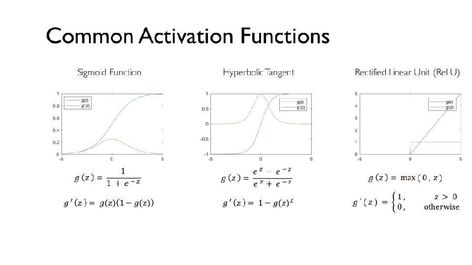
Non Linearity (Re. LU) Re. LU stands for Rectified Linear Unit and is a non-linear operation. Its output is given by:

Non Linearity (Re. LU) Pros • It avoids and rectifies vanishing gradient problem. • Re. Lu is less computationally expensive than tanh and sigmoid because it involves simpler mathematical operations. Cons • One of its limitation is that it should only be used within Hidden layers of a Neural Network Model. • Some gradients can be fragile during training and can die. It can cause a weight update which will makes it never activate on any data point again. Simply saying that Re. Lu could result in Dead Neurons. • In another words, For activations in the region (x<0) of Re. Lu, gradient will be 0 because of which the weights will not get adjusted during descent. That means, those neurons which go into that state will stop responding to variations in error/ input (simply because gradient is 0, nothing changes ). This is called dying Re. Lu problem. • The range of Re. Lu is [0, inf). This means it can blow up the activation.

Leaky Re. LU Leaky. Relu is a variant of Re. LU. Instead of being 0 when z<0, a leaky Re. LU allows a small, non-zero, constant gradient α (Normally, α=0. 01). Pros Leaky Re. LUs are one attempt to fix the “dying Re. LU” problem by having a small negative slope (of 0. 01, or so). Cons As it possess linearity, it can’t be used for the complex Classification. It lags behind the Sigmoid and Tanh for some of the use cases.

Other Activation Functions - Sigmoid takes a real value as input and outputs another value between 0 and 1. It’s easy to work with and has all the nice properties of activation functions: it’s non-linear, continuously differentiable, monotonic, and has a fixed output range.

Other Activation Functions - Tanh squashes a real-valued number to the range [-1, 1]. It’s non-linear. But unlike Sigmoid, its output is zero-centered.

Other Activation Functions - Softmax function calculates the probabilities distribution of the event over ‘n’ different events. In general way of saying, this function will calculate the probabilities of each target class over all possible target classes. Later the calculated probabilities will be helpful for determining the target class for the given inputs.

Pooling Spatial Pooling (also called subsampling or downsampling) reduces the dimensionality of each feature map but retains the most important information. Spatial Pooling can be of different types: Max, Average, Sum etc. In case of Max Pooling, we define a spatial neighborhood (for example, a 2× 2 window) and take the largest element from the rectified feature map within that window. Instead of taking the largest element we could also take the average (Average Pooling) or sum of all elements in that window. In practice, Max Pooling has been shown to work better.

Pooling

Pooling In particular, pooling: • makes the input representations (feature dimension) smaller and more manageable • reduces the number of parameters and computations in the network, therefore, controlling overfitting • makes the network invariant to small transformations, distortions and translations in the input image (a small distortion in input will not change the output of Pooling – since we take the maximum / average value in a local neighborhood). • helps us arrive at an almost scale invariant representation of our image (the exact term is “equivariant”). This is very powerful since we can detect objects in an image no matter where they are located

Fully Connected Layer The Fully Connected layer is a traditional Multi Layer Perceptron that uses a softmax* activation function in the output layer (other classifiers like SVM can also be used). The term “Fully Connected” implies that every neuron in the previous layer is connected to every neuron on the next layer. *Softmax classifiers give you probabilities for each class label. Softmax classifier is a generalization of the binary form of Logistic Regression

Fully Connected Layer The Fully Connected layer is a traditional Multi Layer Perceptron that uses a softmax* activation function in the output layer (other classifiers like SVM can also be used). The term “Fully Connected” implies that every neuron in the previous layer is connected to every neuron on the next layer. *Softmax classifiers give you probabilities for each class label. Softmax classifier is a generalization of the binary form of Logistic Regression

The network

Training the network The overall training process of the Convolution Network may be summarized as below: Step 1: We initialize all filters and parameters / weights with random values Step 2: The network takes a training image as input, goes through the forward propagation step (convolution, Re. LU and pooling operations along with forward propagation in the Fully Connected layer) and finds the output probabilities for each class. Step 3: Calculate the total error at the output layer Step 4: Use Backpropagation to calculate the gradients of the error with respect to all weights in the network and use gradient descent to update all filter values / weights and parameter values to minimize the output error. Step 5: Repeat steps 2 -4 with all images in the training set.

Testing the network When a new (unseen) image is input into the Conv. Net, the network would go through the forward propagation step and output a probability for each class (for a new image, the output probabilities are calculated using the weights which have been optimized to correctly classify all the previous training examples). If our training set is large enough, the network will (hopefully) generalize well to new images and classify them into correct categories.

Testing the network When a new (unseen) image is input into the Conv. Net, the network would go through the forward propagation step and output a probability for each class (for a new image, the output probabilities are calculated using the weights which have been optimized to correctly classify all the previous training examples). If our training set is large enough, the network will (hopefully) generalize well to new images and classify them into correct categories.

Some Network Architectures Le. Net (1990 s): Already covered in this article. 1990 s to 2012: In the years from late 1990 s to early 2010 s convolutional neural network were in incubation. As more and more data and computing power became available, tasks that convolutional neural networks could tackle became more and more interesting. Alex. Net (2012) – In 2012, Alex Krizhevsky (and others) released Alex. Net which was a deeper and much wider version of the Le. Net and won by a large margin the difficult Image. Net Large Scale Visual Recognition Challenge (ILSVRC) in 2012. It was a significant breakthrough with respect to the previous approaches and the current widespread application of CNNs can be attributed to this work. ZF Net (2013) – The ILSVRC 2013 winner was a Convolutional Network from Matthew Zeiler and Rob Fergus. It became known as the ZFNet (short for Zeiler & Fergus Net). It was an improvement on Alex. Net by tweaking the architecture hyperparameters. Goog. Le. Net (2014) – The ILSVRC 2014 winner was a Convolutional Network from Szegedy et al. from Google. Its main contribution was the development of an Inception Module that dramatically reduced the number of parameters in the network (4 M, compared to Alex. Net with 60 M).

Some Network Architectures VGGNet (2014) – The runner-up in ILSVRC 2014 was the network that became known as the VGGNet. Its main contribution was in showing that the depth of the network (number of layers) is a critical component for good performance. Res. Nets (2015) – Residual Network developed by Kaiming He (and others) was the winner of ILSVRC 2015. Res. Nets are currently by far state of the art Convolutional Neural Network models and are the default choice for using Conv. Nets in practice (as of May 2016). Dense. Net (August 2016) – Recently published by Gao Huang (and others), the Densely Connected Convolutional Network has each layer directly connected to every other layer in a feed-forward fashion. The Dense. Net has been shown to obtain significant improvements over previous state-of-the-art architectures on five highly competitive object recognition benchmark tasks.

Some Network Architectures - Parameters Network Number of Parameters Le. Net-5 60000 Alex. Net 60 million VGG-16 138 million Google. Net 5 million (V 1) - 23 million (V 3) Res. Net 50 25 million Dense. Net-190 40 million

Autoencoders The autoencoder tries to learn a function h. W, b(x)≈x. In other words, it is trying to learn an approximation to the identity function, so as to output x^x^ that is similar to xx. Typically used for unsupervised learning

Autoencoders Source : https: //towardsdatascience. com/applied-deep-learning-part-3 -autoencoders-1 c 083 af 4 d 798

Other Deep Learning algorithms Ø Ø Long Short-Term Memory (LSTM) Restricted Boltzmann Machine (RBM) Deep Belief Networks (DBN) Generative Adversarial Nets (GANs)

Deep Learning Frameworks Ø Ø Ø Ø Ø Tensorflow Caffe Py. Torch Mx. Net The Microsoft Cognitive Toolkit/CNTK Chainer Keras Deeplearning 4 j Matlab

Thank you

References http: //ufldl. stanford. edu/tutorial/unsupervised/Autoencoders/ https: //ujjwalkarn. me/2016/08/11/intuitive-explanation-convnets/ http: //introtodeeplearning. com/ http: //www. iro. umontreal. ca/~pift 6266/H 10/notes/deepintro. html https: //ml-cheatsheet. readthedocs. io/en/latest/activation_functions. html https: //www. jeremyjordan. me/convnet-architectures/