Introduction to Data Science Lecture 3 Manipulating Tabular

Introduction to Data Science Lecture 3 Manipulating Tabular Data CS 194 Spring 2014 John Canny based on notes from Michael Franklin, Dan Bruckner, Evan Sparks, Shivaram Venkataraman

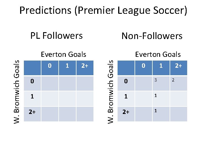
Predictions (Premier League Soccer) PL Followers Non-Followers 0 0 1 2+ Everton Goals W. Bromwich Goals Everton Goals 0 1 0 3 1 1 2+ 2

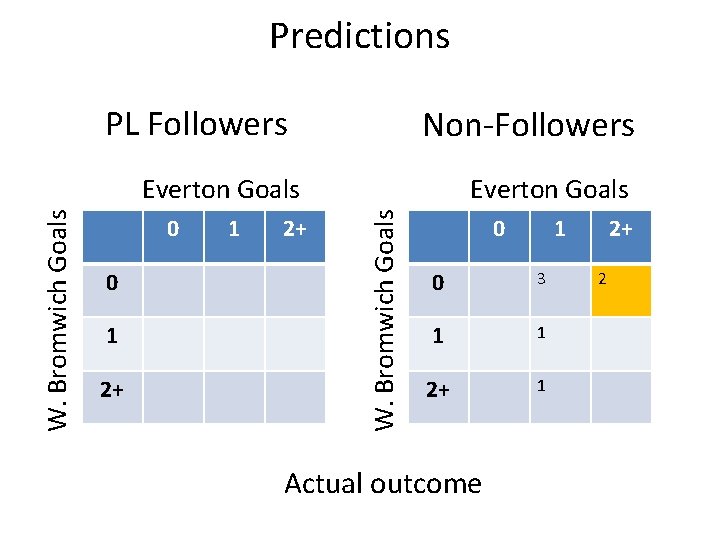
Predictions PL Followers Non-Followers 0 0 1 2+ Everton Goals W. Bromwich Goals Everton Goals 0 1 0 3 1 1 2+ 1 Actual outcome 2+ 2

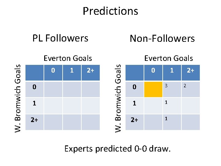
Predictions PL Followers Non-Followers 0 0 1 2+ Everton Goals W. Bromwich Goals Everton Goals 0 1 0 3 1 1 2+ 1 Experts predicted 0 -0 draw. 2+ 2

Watch Cognitive Biases! • People don’t like scoreless games. • People don’t like drawn games. • Beware of using data to justify your opinions vs. giving you answers. Also important: • Don’t overinterpret: there aren’t enough data points to draw firm conclusions on this problem – but you can certainly look for trends and try to confirm them with more data. 5

Outline for this Evening • Wrap-up file storage from last time • Lecture – Data Models, Tables, Structure, etc. – SQL, No. SQL – Schema on Read vs. Schema on Write – Non-Tabular Structures

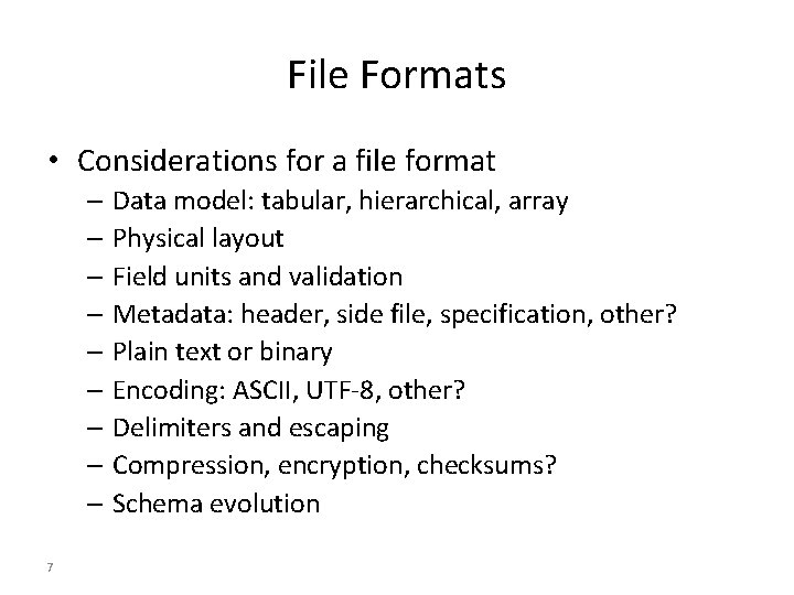
File Formats • Considerations for a file format – Data model: tabular, hierarchical, array – Physical layout – Field units and validation – Metadata: header, side file, specification, other? – Plain text or binary – Encoding: ASCII, UTF-8, other? – Delimiters and escaping – Compression, encryption, checksums? – Schema evolution 7

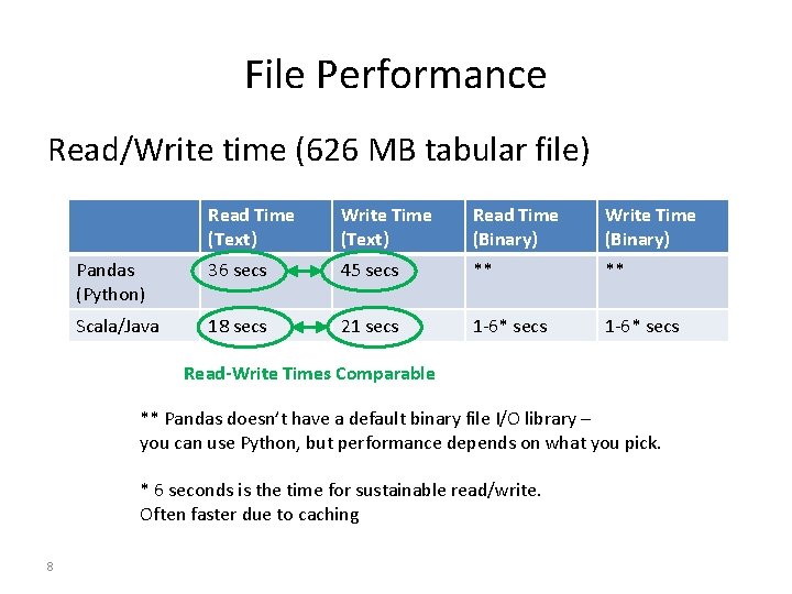
File Performance Read/Write time (626 MB tabular file) Read Time (Text) Write Time (Text) Read Time (Binary) Write Time (Binary) Pandas (Python) 36 secs 45 secs ** ** Scala/Java 18 secs 21 secs 1 -6* secs Read-Write Times Comparable ** Pandas doesn’t have a default binary file I/O library – you can use Python, but performance depends on what you pick. * 6 seconds is the time for sustainable read/write. Often faster due to caching 8

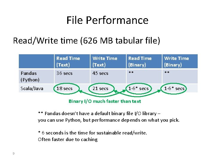
File Performance Read/Write time (626 MB tabular file) Read Time (Text) Write Time (Text) Read Time (Binary) Write Time (Binary) Pandas (Python) 36 secs 45 secs ** ** Scala/Java 18 secs 21 secs 1 -6* secs Binary I/O much faster than text ** Pandas doesn’t have a default binary file I/O library – you can use Python, but performance depends on what you pick. * 6 seconds is the time for sustainable read/write. Often faster due to caching 9

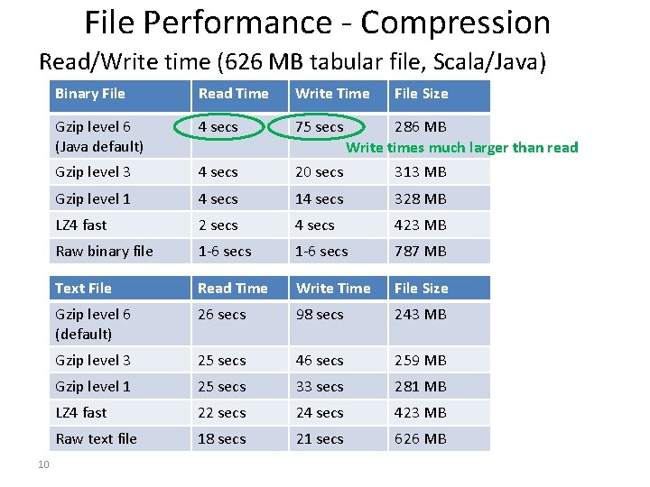
File Performance - Compression Read/Write time (626 MB tabular file, Scala/Java) 10 Binary File Read Time Write Time File Size Gzip level 6 (Java default) 4 secs 75 secs Gzip level 3 4 secs 20 secs 313 MB Gzip level 1 4 secs 14 secs 328 MB LZ 4 fast 2 secs 423 MB Raw binary file 1 -6 secs 787 MB Text File Read Time Write Time File Size Gzip level 6 (default) 26 secs 98 secs 243 MB Gzip level 3 25 secs 46 secs 259 MB Gzip level 1 25 secs 33 secs 281 MB LZ 4 fast 22 secs 24 secs 423 MB Raw text file 18 secs 21 secs 626 MB 286 MB Write times much larger than read

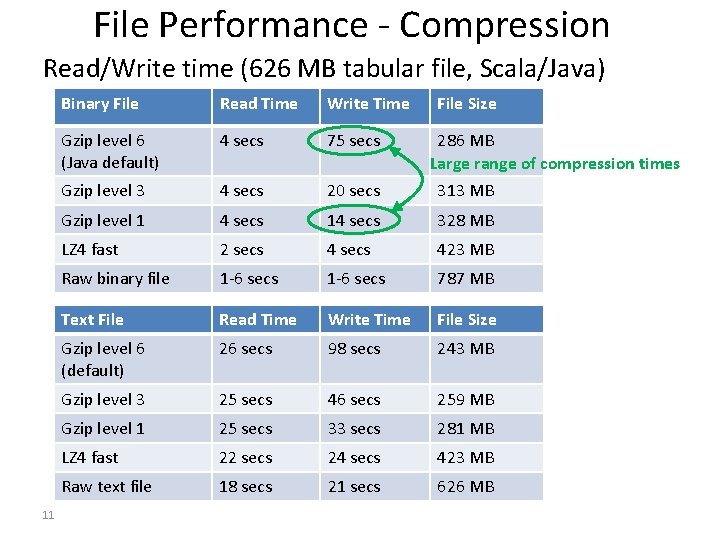
File Performance - Compression Read/Write time (626 MB tabular file, Scala/Java) 11 Binary File Read Time Write Time File Size Gzip level 6 (Java default) 4 secs 75 secs Gzip level 3 4 secs 20 secs 313 MB Gzip level 1 4 secs 14 secs 328 MB LZ 4 fast 2 secs 423 MB Raw binary file 1 -6 secs 787 MB Text File Read Time Write Time File Size Gzip level 6 (default) 26 secs 98 secs 243 MB Gzip level 3 25 secs 46 secs 259 MB Gzip level 1 25 secs 33 secs 281 MB LZ 4 fast 22 secs 24 secs 423 MB Raw text file 18 secs 21 secs 626 MB 286 MB Large range of compression times

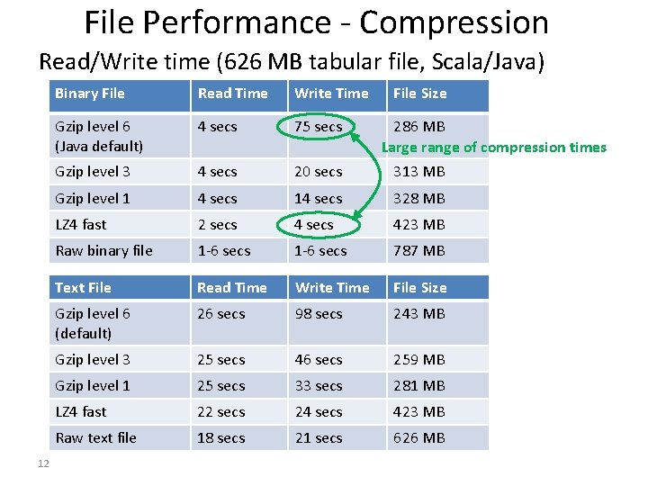
File Performance - Compression Read/Write time (626 MB tabular file, Scala/Java) 12 Binary File Read Time Write Time File Size Gzip level 6 (Java default) 4 secs 75 secs Gzip level 3 4 secs 20 secs 313 MB Gzip level 1 4 secs 14 secs 328 MB LZ 4 fast 2 secs 423 MB Raw binary file 1 -6 secs 787 MB Text File Read Time Write Time File Size Gzip level 6 (default) 26 secs 98 secs 243 MB Gzip level 3 25 secs 46 secs 259 MB Gzip level 1 25 secs 33 secs 281 MB LZ 4 fast 22 secs 24 secs 423 MB Raw text file 18 secs 21 secs 626 MB 286 MB Large range of compression times

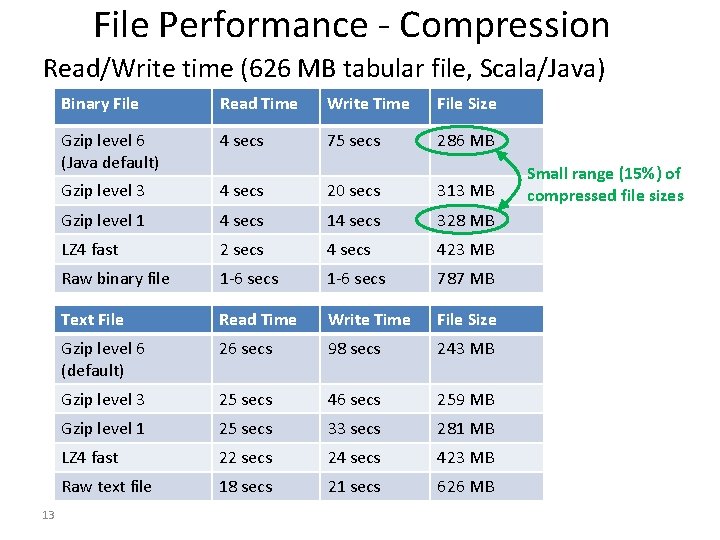
File Performance - Compression Read/Write time (626 MB tabular file, Scala/Java) 13 Binary File Read Time Write Time File Size Gzip level 6 (Java default) 4 secs 75 secs 286 MB Gzip level 3 4 secs 20 secs 313 MB Gzip level 1 4 secs 14 secs 328 MB LZ 4 fast 2 secs 423 MB Raw binary file 1 -6 secs 787 MB Text File Read Time Write Time File Size Gzip level 6 (default) 26 secs 98 secs 243 MB Gzip level 3 25 secs 46 secs 259 MB Gzip level 1 25 secs 33 secs 281 MB LZ 4 fast 22 secs 24 secs 423 MB Raw text file 18 secs 21 secs 626 MB Small range (15%) of compressed file sizes

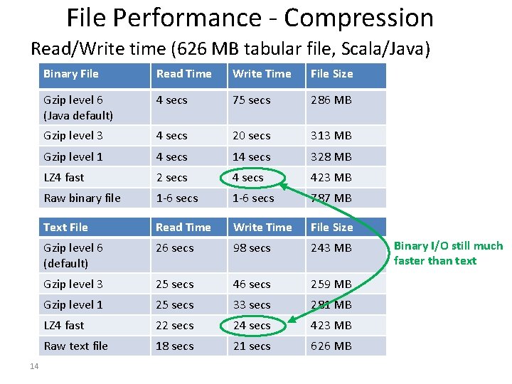
File Performance - Compression Read/Write time (626 MB tabular file, Scala/Java) 14 Binary File Read Time Write Time File Size Gzip level 6 (Java default) 4 secs 75 secs 286 MB Gzip level 3 4 secs 20 secs 313 MB Gzip level 1 4 secs 14 secs 328 MB LZ 4 fast 2 secs 423 MB Raw binary file 1 -6 secs 787 MB Text File Read Time Write Time File Size Gzip level 6 (default) 26 secs 98 secs 243 MB Gzip level 3 25 secs 46 secs 259 MB Gzip level 1 25 secs 33 secs 281 MB LZ 4 fast 22 secs 24 secs 423 MB Raw text file 18 secs 21 secs 626 MB Binary I/O still much faster than text

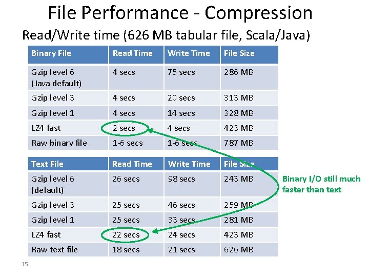
File Performance - Compression Read/Write time (626 MB tabular file, Scala/Java) 15 Binary File Read Time Write Time File Size Gzip level 6 (Java default) 4 secs 75 secs 286 MB Gzip level 3 4 secs 20 secs 313 MB Gzip level 1 4 secs 14 secs 328 MB LZ 4 fast 2 secs 423 MB Raw binary file 1 -6 secs 787 MB Text File Read Time Write Time File Size Gzip level 6 (default) 26 secs 98 secs 243 MB Gzip level 3 25 secs 46 secs 259 MB Gzip level 1 25 secs 33 secs 281 MB LZ 4 fast 22 secs 24 secs 423 MB Raw text file 18 secs 21 secs 626 MB Binary I/O still much faster than text

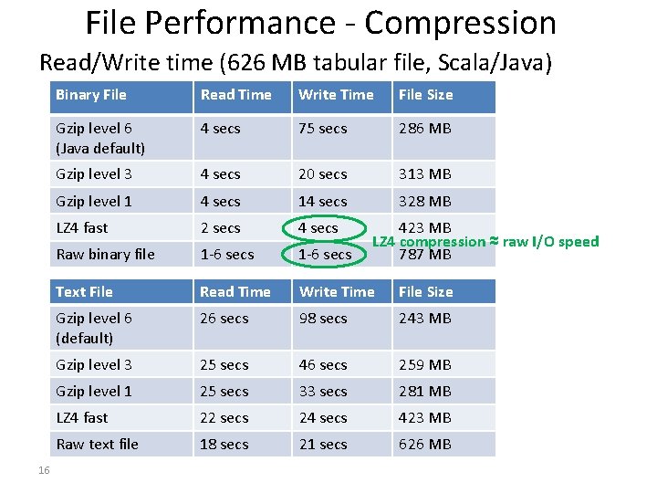
File Performance - Compression Read/Write time (626 MB tabular file, Scala/Java) 16 Binary File Read Time Write Time File Size Gzip level 6 (Java default) 4 secs 75 secs 286 MB Gzip level 3 4 secs 20 secs 313 MB Gzip level 1 4 secs 14 secs 328 MB LZ 4 fast 2 secs 4 secs Raw binary file 1 -6 secs Text File Read Time Write Time File Size Gzip level 6 (default) 26 secs 98 secs 243 MB Gzip level 3 25 secs 46 secs 259 MB Gzip level 1 25 secs 33 secs 281 MB LZ 4 fast 22 secs 24 secs 423 MB Raw text file 18 secs 21 secs 626 MB 423 MB LZ 4 compression ≈ raw I/O speed 787 MB

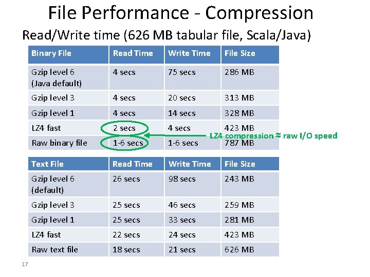
File Performance - Compression Read/Write time (626 MB tabular file, Scala/Java) 17 Binary File Read Time Write Time File Size Gzip level 6 (Java default) 4 secs 75 secs 286 MB Gzip level 3 4 secs 20 secs 313 MB Gzip level 1 4 secs 14 secs 328 MB LZ 4 fast 2 secs 4 secs Raw binary file 1 -6 secs Text File Read Time Write Time File Size Gzip level 6 (default) 26 secs 98 secs 243 MB Gzip level 3 25 secs 46 secs 259 MB Gzip level 1 25 secs 33 secs 281 MB LZ 4 fast 22 secs 24 secs 423 MB Raw text file 18 secs 21 secs 626 MB 423 MB LZ 4 compression ≈ raw I/O speed 787 MB

Data Pipeline Design 10’s. TB 100’s TB Raw Data (Text) 10’s TB TB Binarized, Normalized Data (lossless) TB’s < TB GB’s Key data views (materialized) Clicks, views, Common (often purchases shared) views, e. g. user history. GB’s Final views and queries

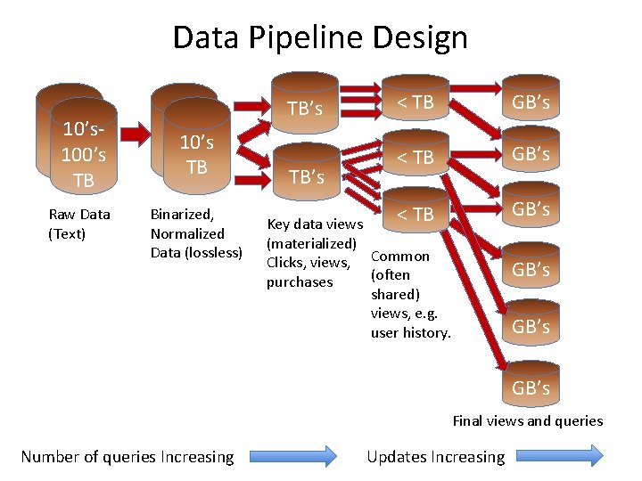
Data Pipeline Design 10’s. TB 100’s TB Raw Data (Text) 10’s TB TB Binarized, Normalized Data (lossless) TB’s < TB GB’s Key data views (materialized) Clicks, views, Common (often purchases shared) views, e. g. user history. GB’s Final views and queries Number of queries Increasing Updates Increasing

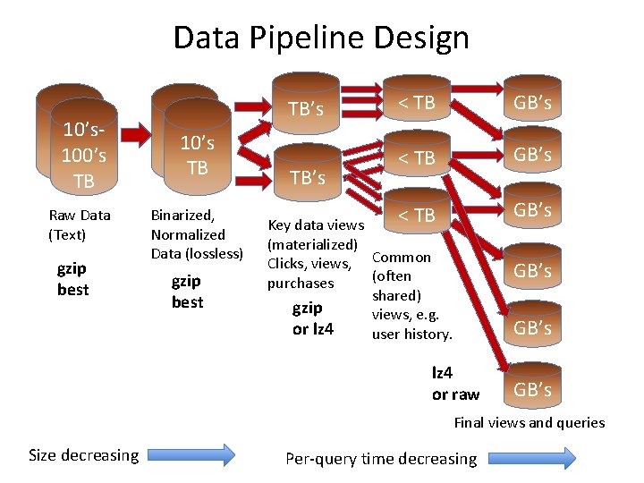
Data Pipeline Design 10’s. TB 100’s TB Raw Data (Text) gzip best 10’s TB TB Binarized, Normalized Data (lossless) gzip best TB’s < TB GB’s Key data views (materialized) Clicks, views, Common (often purchases shared) gzip views, e. g. or lz 4 user history. GB’s lz 4 or raw GB’s Final views and queries Size decreasing Per-query time decreasing

Outline for this Evening • Data Models, Tables, Structure, etc. – SQL – No. SQL – Schema on Read vs. Schema on Write

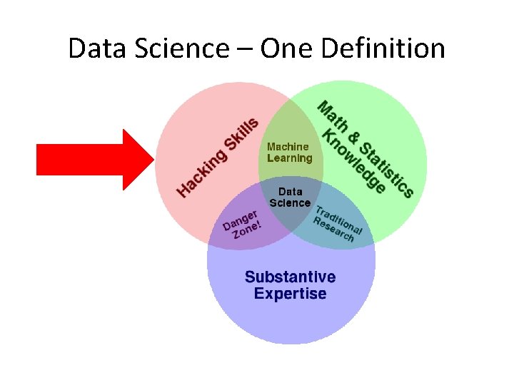
Data Science – One Definition

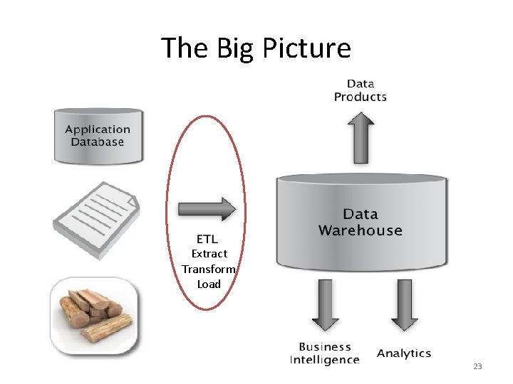
The Big Picture Extract Transform Load 23

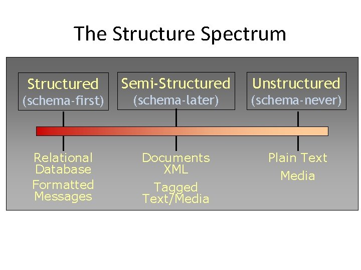
The Structure Spectrum Structured Semi-Structured Unstructured (schema-first) (schema-later) (schema-never) Relational Database Formatted Messages Documents XML Plain Text Tagged Text/Media

Key Concept: Structured Data A data model is a collection of concepts for describing data. A schema is a description of a particular collection of data, using a given data model.

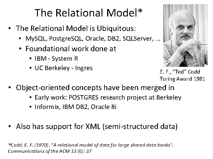
The Relational Model* • The Relational Model is Ubiquitous: • My. SQL, Postgre. SQL, Oracle, DB 2, SQLServer, … • Foundational work done at • IBM - System R • UC Berkeley - Ingres E. F. , “Ted” Codd Turing Award 1981 • Object-oriented concepts have been merged in • Early work: POSTGRES research project at Berkeley • Informix, IBM DB 2, Oracle 8 i • Also has support for XML (semi-structured data) *Codd, E. F. (1970). "A relational model of data for large shared data banks". Communications of the ACM 13 (6): 37

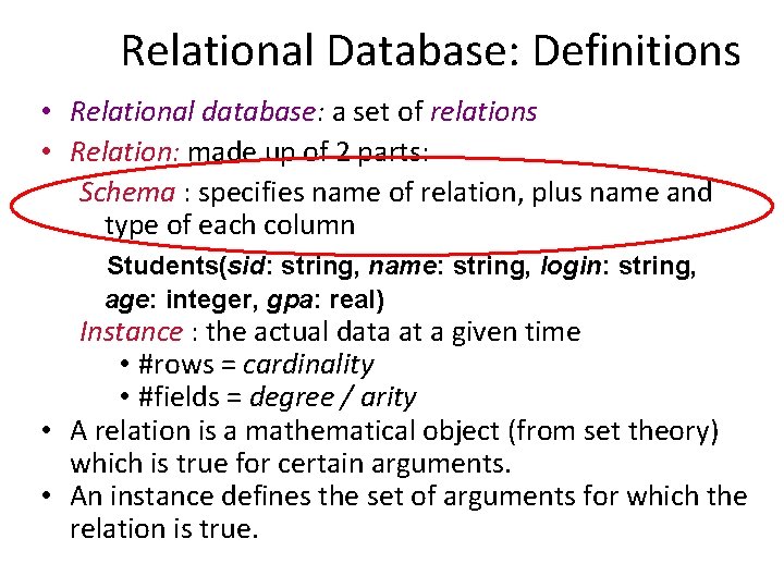
Relational Database: Definitions • Relational database: a set of relations • Relation: made up of 2 parts: Schema : specifies name of relation, plus name and type of each column Students(sid: string, name: string, login: string, age: integer, gpa: real) Instance : the actual data at a given time • #rows = cardinality • #fields = degree / arity • A relation is a mathematical object (from set theory) which is true for certain arguments. • An instance defines the set of arguments for which the relation is true.

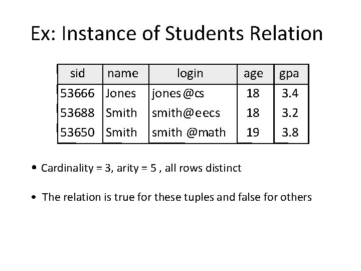
Ex: Instance of Students Relation sid 53666 53688 53650 name login Jones jones@cs Smith smith@eecs Smith smith @math age 18 18 19 gpa 3. 4 3. 2 3. 8 • Cardinality = 3, arity = 5 , all rows distinct • The relation is true for these tuples and false for others

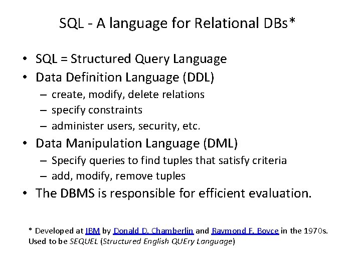
SQL - A language for Relational DBs* • SQL = Structured Query Language • Data Definition Language (DDL) – create, modify, delete relations – specify constraints – administer users, security, etc. • Data Manipulation Language (DML) – Specify queries to find tuples that satisfy criteria – add, modify, remove tuples • The DBMS is responsible for efficient evaluation. * Developed at IBM by Donald D. Chamberlin and Raymond F. Boyce in the 1970 s. Used to be SEQUEL (Structured English QUEry Language)

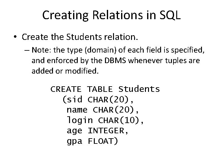
Creating Relations in SQL • Create the Students relation. – Note: the type (domain) of each field is specified, and enforced by the DBMS whenever tuples are added or modified. CREATE TABLE Students (sid CHAR(20), name CHAR(20), login CHAR(10), age INTEGER, gpa FLOAT)

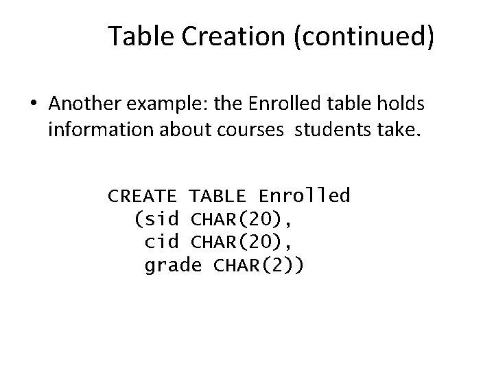
Table Creation (continued) • Another example: the Enrolled table holds information about courses students take. CREATE TABLE Enrolled (sid CHAR(20), cid CHAR(20), grade CHAR(2))

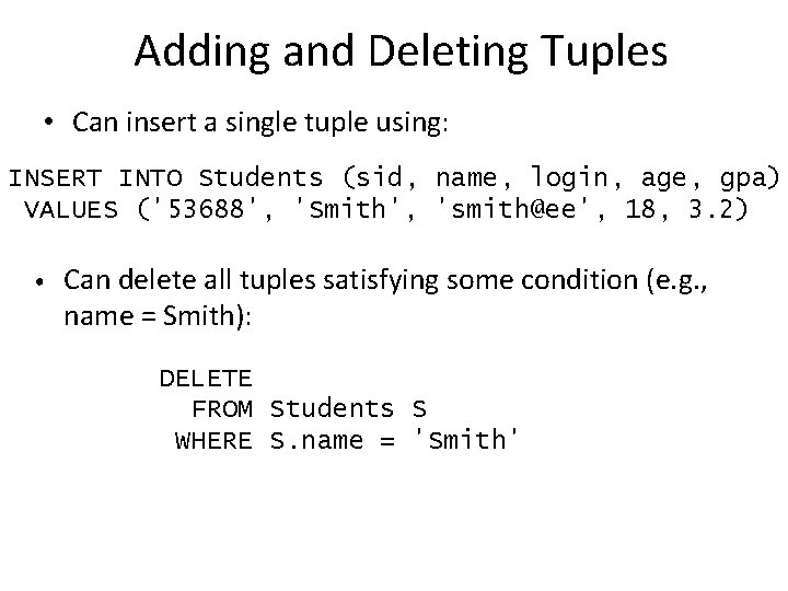
Adding and Deleting Tuples • Can insert a single tuple using: INSERT INTO Students (sid, name, login, age, gpa) VALUES ('53688', 'Smith', 'smith@ee', 18, 3. 2) • Can delete all tuples satisfying some condition (e. g. , name = Smith): DELETE FROM Students S WHERE S. name = 'Smith'

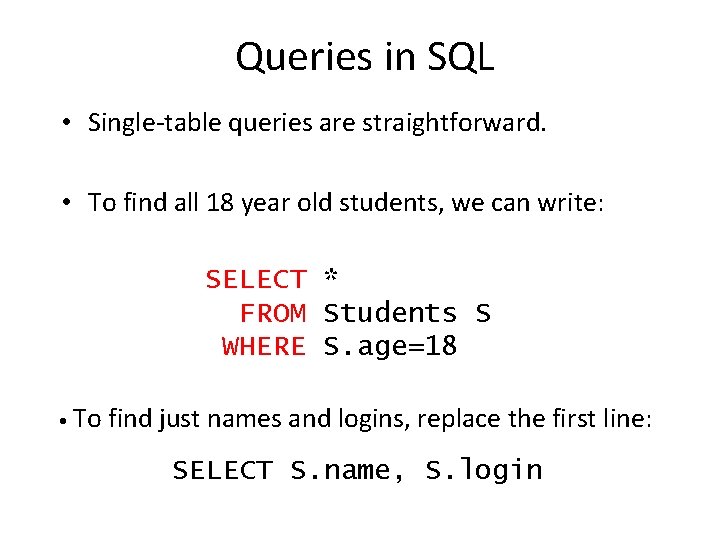
Queries in SQL • Single-table queries are straightforward. • To find all 18 year old students, we can write: SELECT * FROM Students S WHERE S. age=18 • To find just names and logins, replace the first line: SELECT S. name, S. login

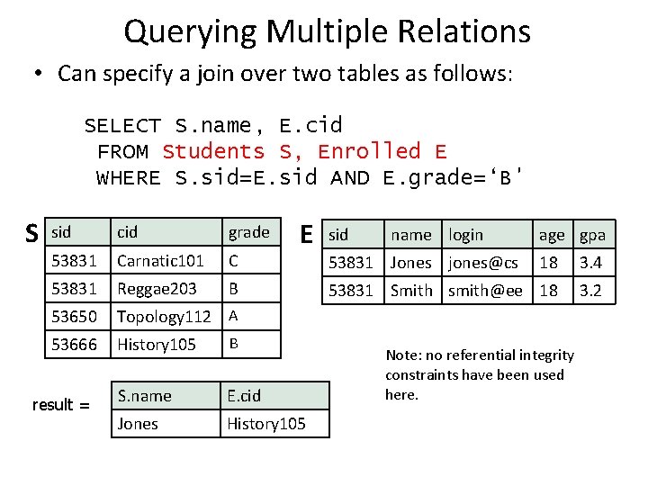
Querying Multiple Relations • Can specify a join over two tables as follows: SELECT S. name, E. cid FROM Students S, Enrolled E WHERE S. sid=E. sid AND E. grade=‘B' S E sid cid grade 53831 Carnatic 101 C 53831 Reggae 203 B 53650 Topology 112 A 53666 History 105 B S. name E. cid Jones History 105 result = sid name login 53831 Jones jones@cs age gpa 18 3. 4 53831 Smith smith@ee 18 3. 2 Note: no referential integrity constraints have been used here.

Basic SQL Query SELECT FROM WHERE [DISTINCT] target-list relation-list qualification • relation-list : A list of relation names • possibly with a range-variable after each name • target-list : A list of attributes of tables in relation-list • qualification : Comparisons combined using AND, OR and NOT. • Comparisons are Attr op const or Attr 1 op Attr 2, where op is one of =≠<>≤≥ • DISTINCT: optional keyword indicating that the answer should not contain duplicates. • In SQL SELECT, the default is that duplicates are not eliminated! (Result is called a “multiset”)

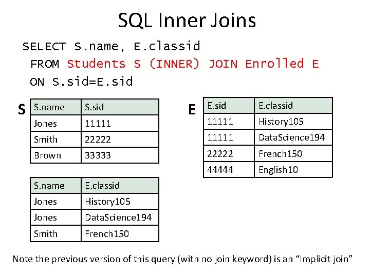
SQL Inner Joins SELECT S. name, E. classid FROM Students S (INNER) JOIN Enrolled E ON S. sid=E. sid S E E. sid E. classid 11111 History 105 22222 11111 Data. Science 194 33333 22222 French 150 44444 English 10 S. name S. sid Jones 11111 Smith Brown S. name E. classid Jones History 105 Jones Data. Science 194 Smith French 150 Note the previous version of this query (with no join keyword) is an “Implicit join”

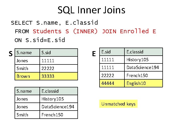
SQL Inner Joins SELECT S. name, E. classid FROM Students S (INNER) JOIN Enrolled E ON S. sid=E. sid S E E. sid E. classid 11111 History 105 22222 11111 Data. Science 194 33333 22222 French 150 44444 English 10 S. name S. sid Jones 11111 Smith Brown S. name E. classid Jones History 105 Jones Data. Science 194 Smith French 150 Unmatched keys

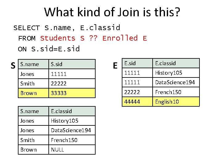
What kind of Join is this? SELECT S. name, E. classid FROM Students S ? ? Enrolled E ON S. sid=E. sid S E E. sid E. classid 11111 History 105 22222 11111 Data. Science 194 33333 22222 French 150 44444 English 10 S. name S. sid Jones 11111 Smith Brown S. name E. classid Jones History 105 Jones Data. Science 194 Smith French 150 Brown NULL

SQL Joins SELECT S. name, E. classid FROM Students S LEFT OUTER JOIN Enrolled E ON S. sid=E. sid S E E. sid E. classid 11111 History 105 22222 11111 Data. Science 194 33333 22222 French 150 44444 English 10 S. name S. sid Jones 11111 Smith Brown S. name E. classid Jones History 105 Jones Data. Science 194 Smith French 150 Brown NULL

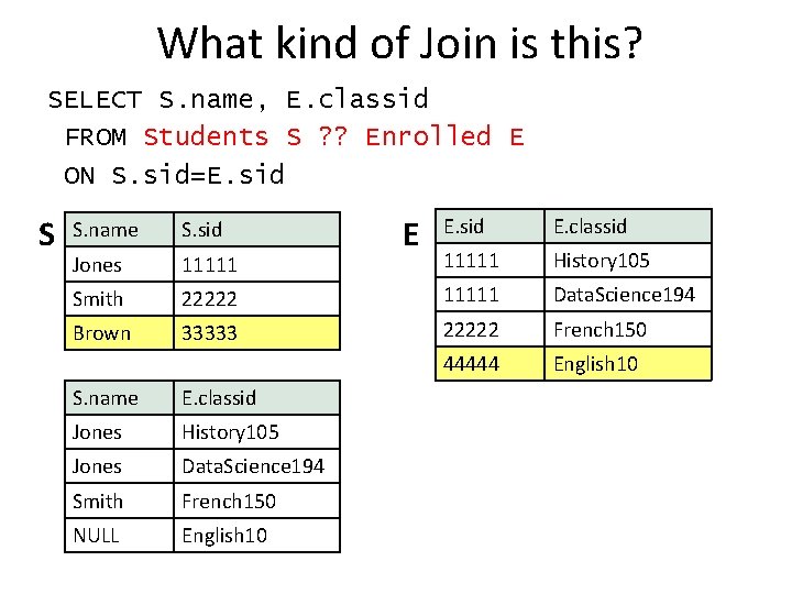
What kind of Join is this? SELECT S. name, E. classid FROM Students S ? ? Enrolled E ON S. sid=E. sid S E E. sid E. classid 11111 History 105 22222 11111 Data. Science 194 33333 22222 French 150 44444 English 10 S. name S. sid Jones 11111 Smith Brown S. name E. classid Jones History 105 Jones Data. Science 194 Smith French 150 NULL English 10

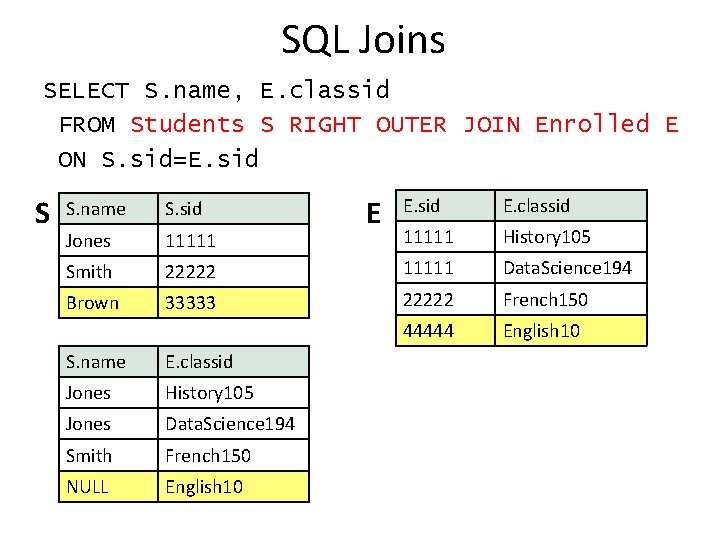
SQL Joins SELECT S. name, E. classid FROM Students S RIGHT OUTER JOIN Enrolled E ON S. sid=E. sid S E E. sid E. classid 11111 History 105 22222 11111 Data. Science 194 33333 22222 French 150 44444 English 10 S. name S. sid Jones 11111 Smith Brown S. name E. classid Jones History 105 Jones Data. Science 194 Smith French 150 NULL English 10

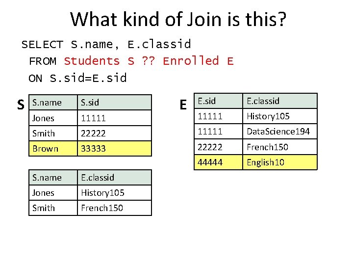
What kind of Join is this? SELECT S. name, E. classid FROM Students S ? ? Enrolled E ON S. sid=E. sid S E E. sid E. classid 11111 History 105 22222 11111 Data. Science 194 33333 22222 French 150 44444 English 10 S. name S. sid Jones 11111 Smith Brown S. name E. classid Jones History 105 Smith French 150

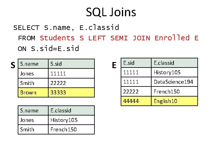
SQL Joins SELECT S. name, E. classid FROM Students S LEFT SEMI JOIN Enrolled E ON S. sid=E. sid S E E. sid E. classid 11111 History 105 22222 11111 Data. Science 194 33333 22222 French 150 44444 English 10 S. name S. sid Jones 11111 Smith Brown S. name E. classid Jones History 105 Smith French 150

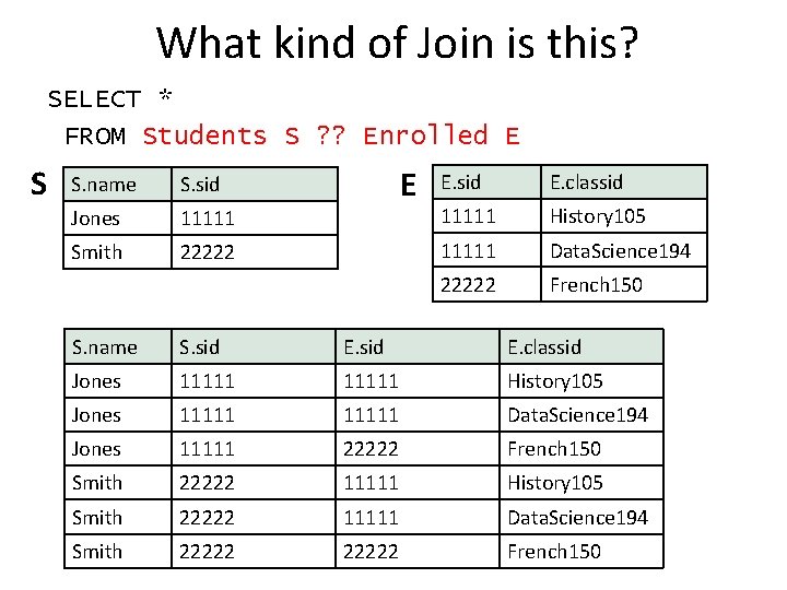
What kind of Join is this? SELECT * FROM Students S ? ? Enrolled E S S. name S. sid Jones 11111 Smith 22222 E E. sid E. classid 11111 History 105 11111 Data. Science 194 22222 French 150 S. name S. sid E. classid Jones 11111 History 105 Jones 11111 Data. Science 194 Jones 11111 22222 French 150 Smith 22222 11111 History 105 Smith 22222 11111 Data. Science 194 Smith 22222 French 150

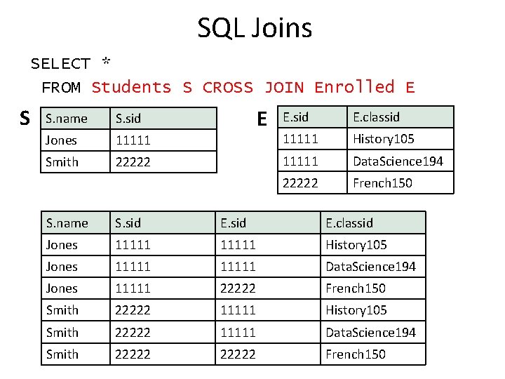
SQL Joins SELECT * FROM Students S CROSS JOIN Enrolled E S S. name S. sid Jones 11111 Smith 22222 E E. sid E. classid 11111 History 105 11111 Data. Science 194 22222 French 150 S. name S. sid E. classid Jones 11111 History 105 Jones 11111 Data. Science 194 Jones 11111 22222 French 150 Smith 22222 11111 History 105 Smith 22222 11111 Data. Science 194 Smith 22222 French 150

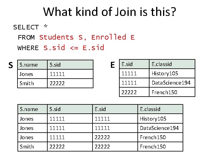
What kind of Join is this? SELECT * FROM Students S, Enrolled E WHERE S. sid <= E. sid S S. name S. sid Jones 11111 Smith 22222 E E. sid E. classid 11111 History 105 11111 Data. Science 194 22222 French 150 S. name S. sid E. classid Jones 11111 History 105 Jones 11111 Data. Science 194 Jones 11111 22222 French 150 Smith 22222 French 150

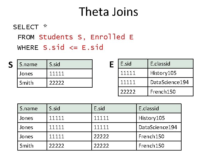
Theta Joins SELECT * FROM Students S, Enrolled E WHERE S. sid <= E. sid S S. name S. sid Jones 11111 Smith 22222 E E. sid E. classid 11111 History 105 11111 Data. Science 194 22222 French 150 S. name S. sid E. classid Jones 11111 History 105 Jones 11111 Data. Science 194 Jones 11111 22222 French 150 Smith 22222 French 150

OTHER “TABLE-LIKE” DATA MODELS

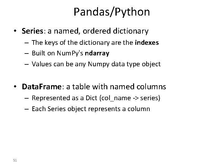
Pandas/Python • Series: a named, ordered dictionary – The keys of the dictionary are the indexes – Built on Num. Py’s ndarray – Values can be any Numpy data type object • Data. Frame: a table with named columns – Represented as a Dict (col_name -> series) – Each Series object represents a column 51

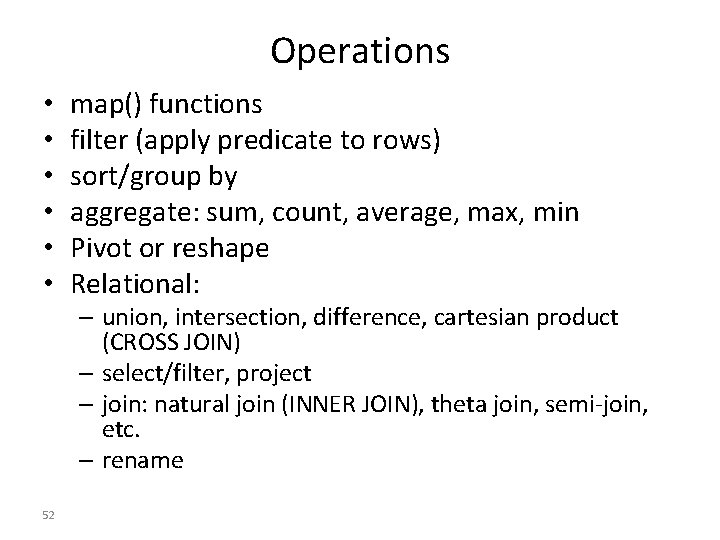
Operations • • • map() functions filter (apply predicate to rows) sort/group by aggregate: sum, count, average, max, min Pivot or reshape Relational: – union, intersection, difference, cartesian product (CROSS JOIN) – select/filter, project – join: natural join (INNER JOIN), theta join, semi-join, etc. – rename 52

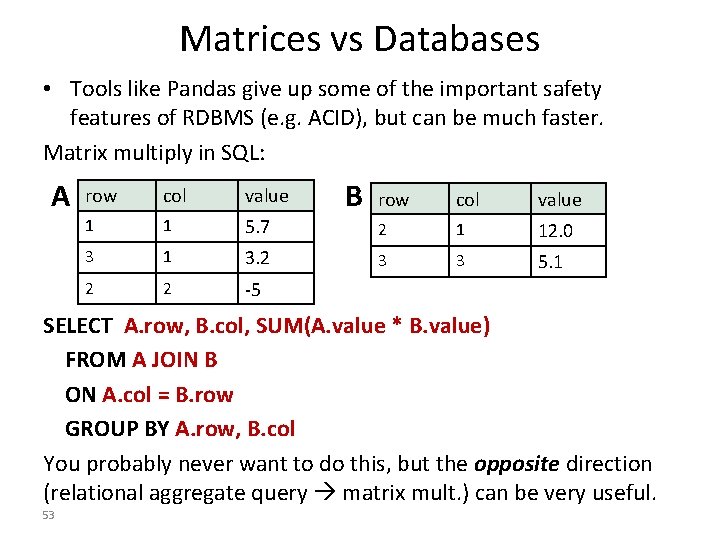
Matrices vs Databases • Tools like Pandas give up some of the important safety features of RDBMS (e. g. ACID), but can be much faster. Matrix multiply in SQL: A row col value 1 1 5. 7 3 1 3. 2 2 2 -5 B row col value 2 1 12. 0 3 3 5. 1 SELECT A. row, B. col, SUM(A. value * B. value) FROM A JOIN B ON A. col = B. row GROUP BY A. row, B. col You probably never want to do this, but the opposite direction (relational aggregate query matrix mult. ) can be very useful. 53

5 min break

What’s Wrong with Tables? • Too limited in structure? • Too rigid? • Too old fashioned?

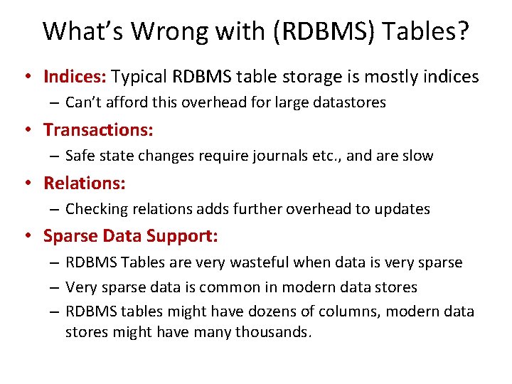
What’s Wrong with (RDBMS) Tables? • Indices: Typical RDBMS table storage is mostly indices – Can’t afford this overhead for large datastores • Transactions: – Safe state changes require journals etc. , and are slow • Relations: – Checking relations adds further overhead to updates • Sparse Data Support: – RDBMS Tables are very wasteful when data is very sparse – Very sparse data is common in modern data stores – RDBMS tables might have dozens of columns, modern data stores might have many thousands.

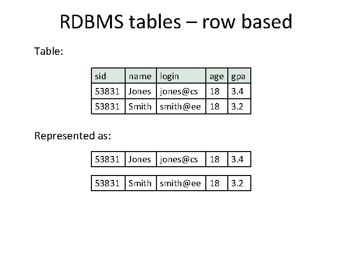
RDBMS tables – row based Table: sid name login 53831 Jones jones@cs age gpa 18 3. 4 53831 Smith smith@ee 18 3. 2 Represented as: 53831 Jones jones@cs 18 3. 4 53831 Smith smith@ee 18 3. 2

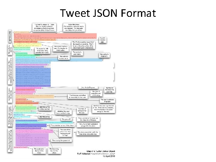
Tweet JSON Format

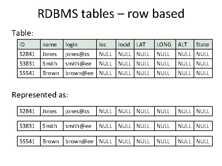
RDBMS tables – row based Table: ID name login loc 52841 Jones jones@cs 53831 Smith smith@ee 55541 Brown locid LAT LONG ALT State NULL NULL NULL brown@ee NULL NULL Represented as: 52841 Jones jones@cs NULL NULL 53831 Smith smith@ee NULL NULL 55541 Brown brown@ee NULL NULL

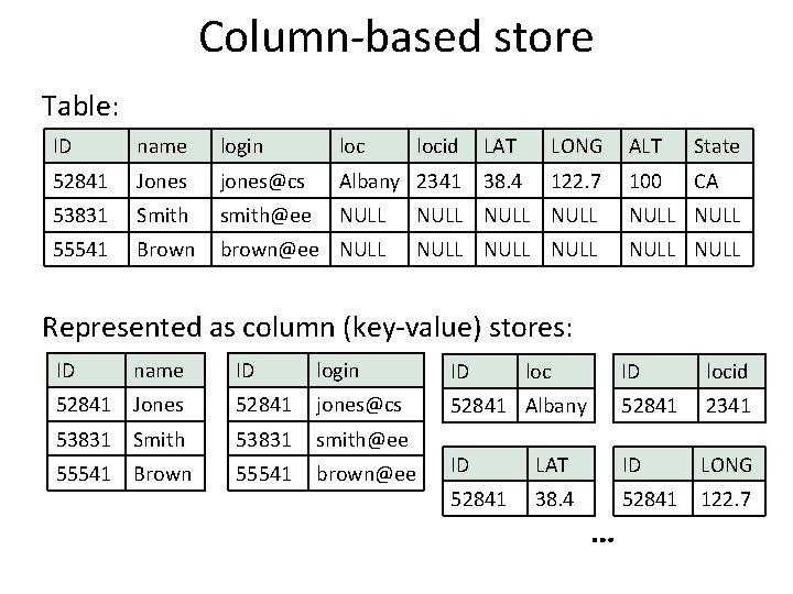
Column-based store Table: ID name login locid LAT LONG ALT State 52841 Jones jones@cs Albany 2341 38. 4 122. 7 100 CA 53831 Smith smith@ee NULL NULL 55541 Brown brown@ee NULL NULL Represented as column (key-value) stores: ID name ID login ID 52841 Jones 52841 jones@cs 53831 Smith 53831 smith@ee 55541 Brown 55541 brown@ee loc ID locid 52841 Albany 52841 2341 ID LAT ID LONG 52841 38. 4 52841 122. 7 …

BEYOND TABLES

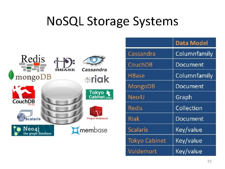
No. SQL Storage Systems 62

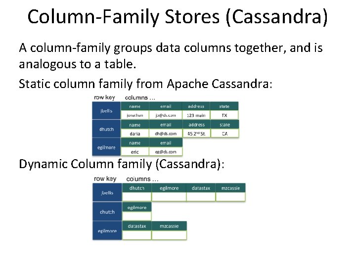
Column-Family Stores (Cassandra) A column-family groups data columns together, and is analogous to a table. Static column family from Apache Cassandra: Dynamic Column family (Cassandra):

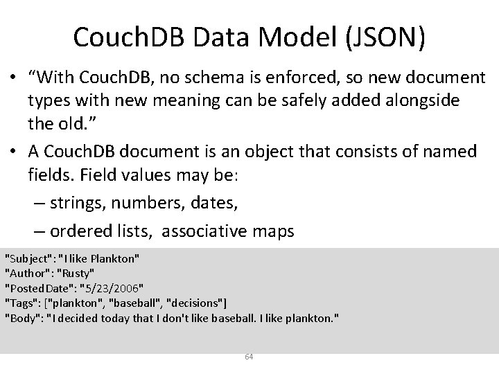
Couch. DB Data Model (JSON) • “With Couch. DB, no schema is enforced, so new document types with new meaning can be safely added alongside the old. ” • A Couch. DB document is an object that consists of named fields. Field values may be: – strings, numbers, dates, – ordered lists, associative maps "Subject": "I like Plankton" "Author": "Rusty" "Posted. Date": "5/23/2006" "Tags": ["plankton", "baseball", "decisions"] "Body": "I decided today that I don't like baseball. I like plankton. " 64

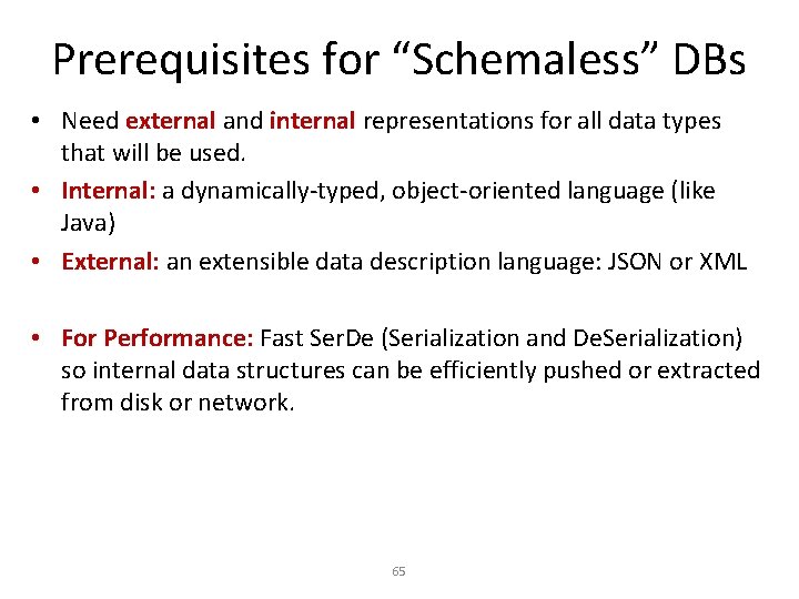
Prerequisites for “Schemaless” DBs • Need external and internal representations for all data types that will be used. • Internal: a dynamically-typed, object-oriented language (like Java) • External: an extensible data description language: JSON or XML • For Performance: Fast Ser. De (Serialization and De. Serialization) so internal data structures can be efficiently pushed or extracted from disk or network. 65

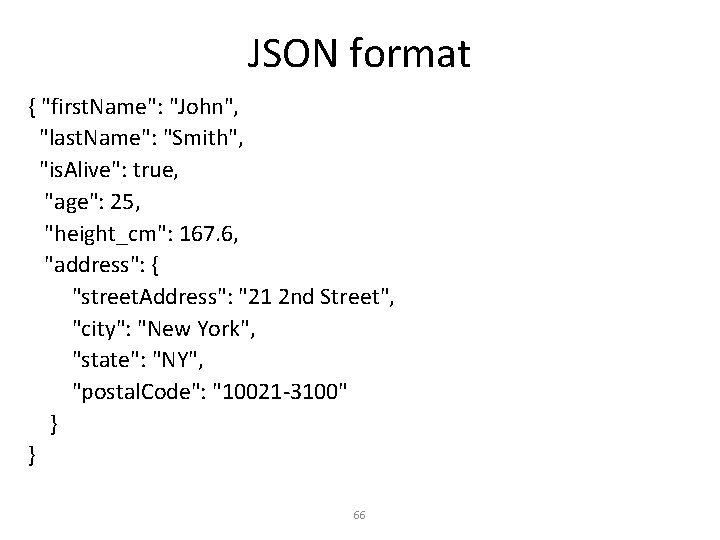
JSON format { "first. Name": "John", "last. Name": "Smith", "is. Alive": true, "age": 25, "height_cm": 167. 6, "address": { "street. Address": "21 2 nd Street", "city": "New York", "state": "NY", "postal. Code": "10021 -3100" } } 66

Prerequisites for “Schemaless” DBs • JSON includes named fields in a tree structure. Primitive types (e. g. string, number, boolean, …) are implicit. • We can read JSON data (or XML) and automatically create internal representations for complex data. • Using the field names and object structure, we can query these objects once loaded. 67

Pig • Started at Yahoo! Research • Runs about 50% of Yahoo!’s jobs • Features: – Expresses sequences of Map. Reduce jobs – Data model: nested “bags” of items • Schema is optional – Provides relational (SQL) operators (JOIN, GROUP BY, etc) – Easy to plug in Java functions

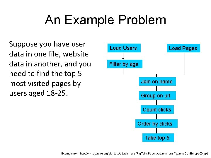
An Example Problem Suppose you have user data in one file, website data in another, and you need to find the top 5 most visited pages by users aged 18 -25. Load Users Load Pages Filter by age Join on name Group on url Count clicks Order by clicks Take top 5 Example from http: //wiki. apache. org/pig-data/attachments/Pig. Talks. Papers/attachments/Apache. Con. Europe 09. ppt

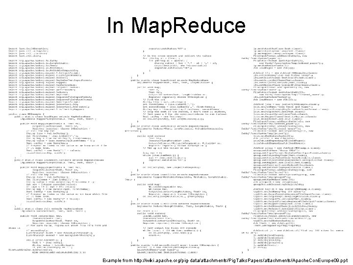
In Map. Reduce Example from http: //wiki. apache. org/pig-data/attachments/Pig. Talks. Papers/attachments/Apache. Con. Europe 09. ppt

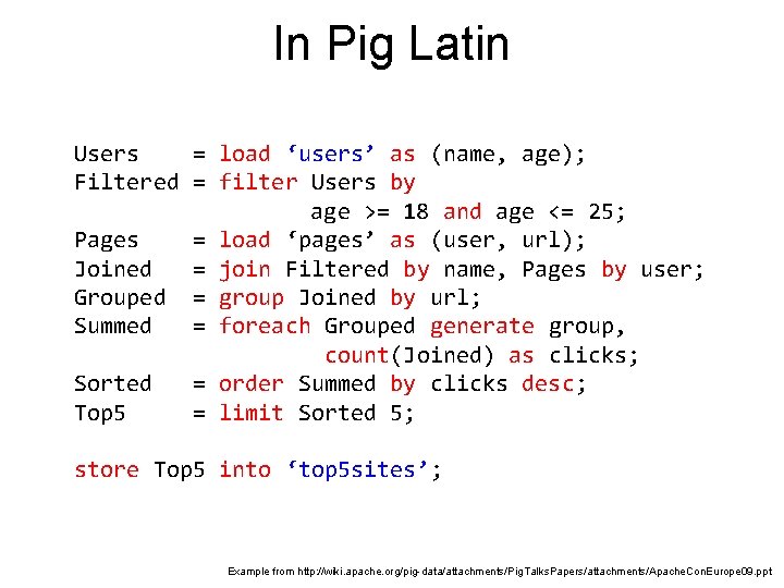
In Pig Latin Users = load ‘users’ as (name, age); Filtered = filter Users by age >= 18 and age <= 25; Pages = load ‘pages’ as (user, url); Joined = join Filtered by name, Pages by user; Grouped = group Joined by url; Summed = foreach Grouped generate group, count(Joined) as clicks; Sorted = order Summed by clicks desc; Top 5 = limit Sorted 5; store Top 5 into ‘top 5 sites’; Example from http: //wiki. apache. org/pig-data/attachments/Pig. Talks. Papers/attachments/Apache. Con. Europe 09. ppt

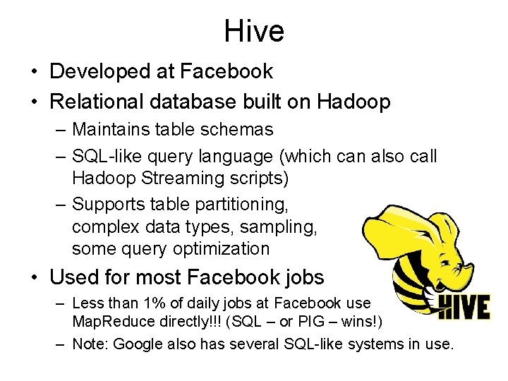
Hive • Developed at Facebook • Relational database built on Hadoop – Maintains table schemas – SQL-like query language (which can also call Hadoop Streaming scripts) – Supports table partitioning, complex data types, sampling, some query optimization • Used for most Facebook jobs – Less than 1% of daily jobs at Facebook use Map. Reduce directly!!! (SQL – or PIG – wins!) – Note: Google also has several SQL-like systems in use.

DATASPACES – WHAT ARE THEY? 73

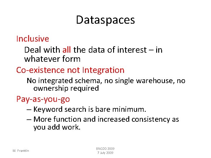
Dataspaces Inclusive Deal with all the data of interest – in whatever form Co-existence not Integration No integrated schema, no single warehouse, no ownership required Pay-as-you-go – Keyword search is bare minimum. – More function and increased consistency as you add work. M. Franklin BNCOD 2009 7 July 2009

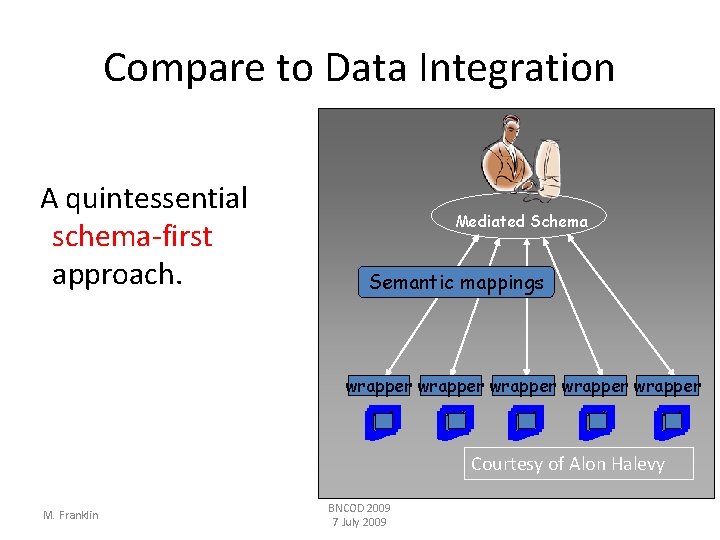
Compare to Data Integration A quintessential schema-first approach. Mediated Schema Semantic mappings wrapper wrapper Courtesy of Alon Halevy M. Franklin BNCOD 2009 7 July 2009

Whither Structured Data? • Conventional Wisdom: only 20% of data is structured. • Decreasing due to: – Consumer applications – Enterprise search – Media applications M. Franklin BNCOD 2009 7 July 2009

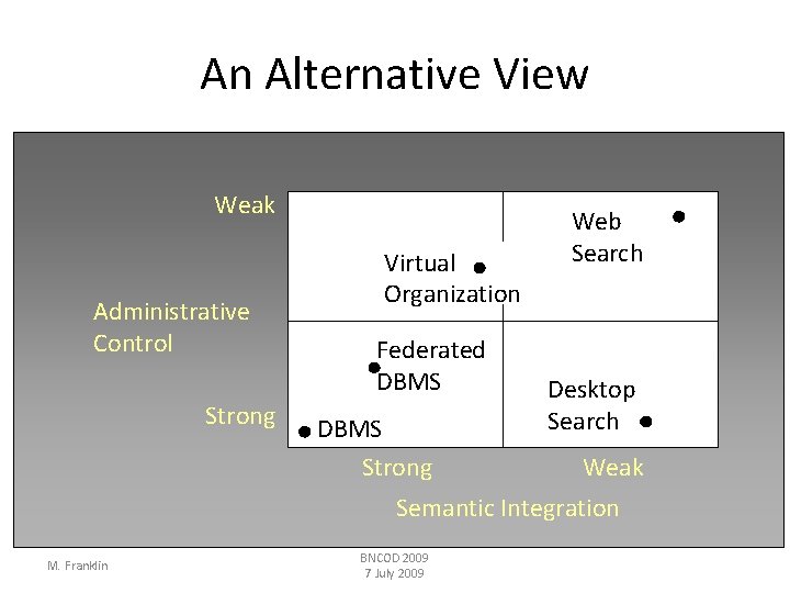
An Alternative View Weak Administrative Control Strong Virtual Organization Federated DBMS Strong Web Search Desktop Search Weak Semantic Integration M. Franklin BNCOD 2009 7 July 2009

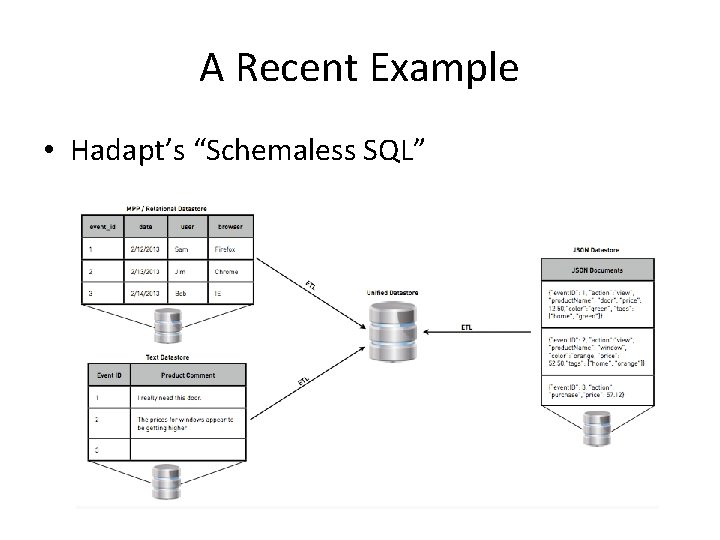
A Recent Example • Hadapt’s “Schemaless SQL”

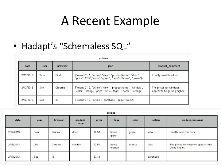
A Recent Example • Hadapt’s “Schemaless SQL”

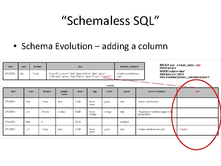
“Schemaless SQL” • Schema Evolution – adding a column

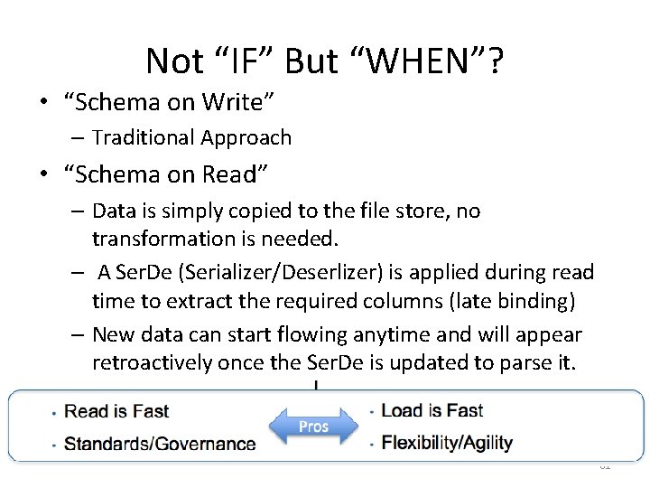
Not “IF” But “WHEN”? • “Schema on Write” – Traditional Approach • “Schema on Read” – Data is simply copied to the file store, no transformation is needed. – A Ser. De (Serializer/Deserlizer) is applied during read time to extract the required columns (late binding) – New data can start flowing anytime and will appear retroactively once the Ser. De is updated to parse it. 81

Summary • Data Models, Tables, Structure, etc. – SQL – No. SQL – Schema on Read vs. Schema on Write • Pandas lab on Wednesday