Introduction to Data Mining and Data Warehousing Muhammad

Introduction to Data Mining and Data Warehousing Muhammad Ali Yousuf DSC – ITM Friday, 9 th May 2003

Data Warehousing and OLAP Technology for Data Mining - I l What l. A is a data warehouse? multi-dimensional data model l Data warehouse architecture l Data warehouse implementation 2

Data Warehousing and OLAP Technology for Data Mining - II l From data warehousing to data mining l Motivation: Why data mining? l What is data mining? l Data Mining: On what kind of data? 3

Data Warehousing and OLAP Technology for Data Mining - III l Data l Are mining functionality all the patterns interesting? l Classification l Major of data mining systems issues in data mining 4

What Is Data Warehouse? l Defined in many different ways, but not rigorously. – A decision support database that is maintained separately from the organization’s operational database. – Support information processing by providing a solid platform of consolidated, historical data for analysis. 5

What Is Data Warehouse? l “A data warehouse is a subject-oriented, integrated, time-variant, and nonvolatile collection of data in support of management’s decision-making process. ” - W. H. Inmon. 6

What Is Data Warehouse? l Data warehousing: – The process of constructing and using data warehouses. 7

Data Warehouse - subject-oriented l Organized around major subjects, such as customer, product, sales. 8

Data Warehouse - subject-oriented l Focusing on the modeling and analysis of data for decision makers, not on daily operations or transaction processing. l Provide a simple and concise view around particular subject issues by excluding data that are not useful in the decision support process. 9

Data Warehouse—integrated l Constructed by integrating multiple, heterogeneous data sources. – Relational databases, flat files, on-line transaction records. l Data cleaning and data integration techniques are applied. – Ensure consistency in naming conventions, encoding structures, attribute measures, etc. Among different data sources. • E. G. , Hotel price: currency, tax, breakfast covered, etc. – When data is moved to the warehouse, it is converted. 10

Data Warehouse—Time Variant l The time horizon for the data warehouse is significantly longer than that of operational systems. – Operational database: current value data. – Data warehouse data: provide information from a historical perspective (e. g. , Past 5 -10 years). 11

Data Warehouse—Time Variant l Every key structure in the data warehouse. – Contains an element of time, explicitly or implicitly. – But the key of operational data may or may not contain “time element”. 12

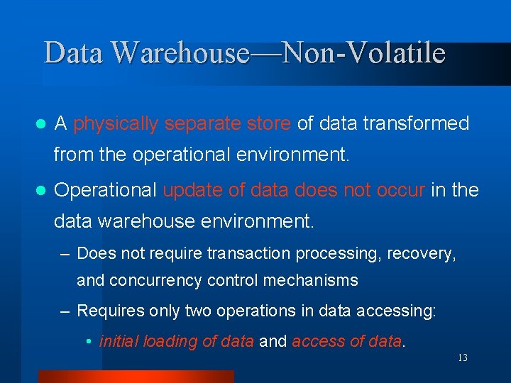
Data Warehouse—Non-Volatile l A physically separate store of data transformed from the operational environment. l Operational update of data does not occur in the data warehouse environment. – Does not require transaction processing, recovery, and concurrency control mechanisms – Requires only two operations in data accessing: • initial loading of data and access of data. 13

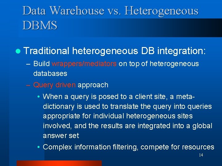
Data Warehouse vs. Heterogeneous DBMS l Traditional heterogeneous DB integration: – Build wrappers/mediators on top of heterogeneous databases – Query driven approach • When a query is posed to a client site, a metadictionary is used to translate the query into queries appropriate for individual heterogeneous sites involved, and the results are integrated into a global answer set • Complex information filtering, compete for resources 14

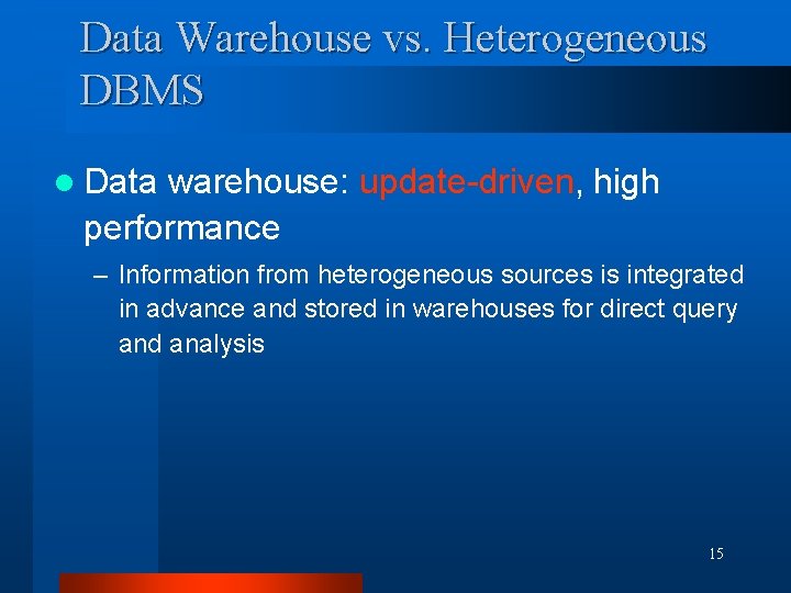
Data Warehouse vs. Heterogeneous DBMS l Data warehouse: update-driven, high performance – Information from heterogeneous sources is integrated in advance and stored in warehouses for direct query and analysis 15

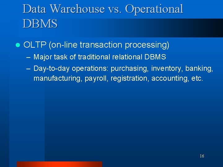
Data Warehouse vs. Operational DBMS l OLTP (on-line transaction processing) – Major task of traditional relational DBMS – Day-to-day operations: purchasing, inventory, banking, manufacturing, payroll, registration, accounting, etc. 16

Data Warehouse vs. Operational DBMS l OLAP (on-line analytical processing) – Major task of data warehouse system – Data analysis and decision making 17

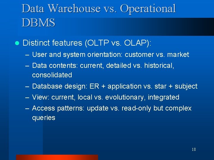
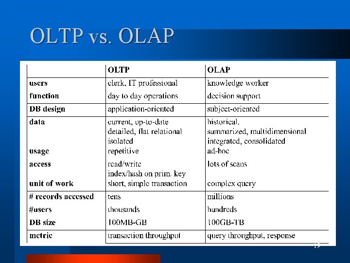
Data Warehouse vs. Operational DBMS l Distinct features (OLTP vs. OLAP): – User and system orientation: customer vs. market – Data contents: current, detailed vs. historical, consolidated – Database design: ER + application vs. star + subject – View: current, local vs. evolutionary, integrated – Access patterns: update vs. read-only but complex queries 18

OLTP vs. OLAP 19

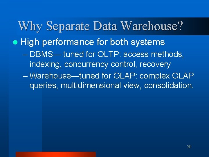
Why Separate Data Warehouse? l High performance for both systems – DBMS— tuned for OLTP: access methods, indexing, concurrency control, recovery – Warehouse—tuned for OLAP: complex OLAP queries, multidimensional view, consolidation. 20

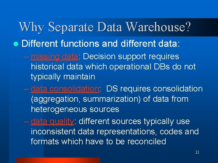
Why Separate Data Warehouse? l Different functions and different data: – missing data: Decision support requires historical data which operational DBs do not typically maintain – data consolidation: DS requires consolidation (aggregation, summarization) of data from heterogeneous sources – data quality: different sources typically use inconsistent data representations, codes and formats which have to be reconciled 21

A Multi-dimensional Data Model 22

From Tables and Spreadsheets to Data Cubes l A data warehouse is based on a multidimensional data model which views data in the form of a data cube 23

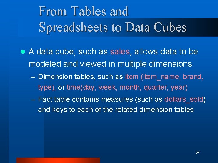
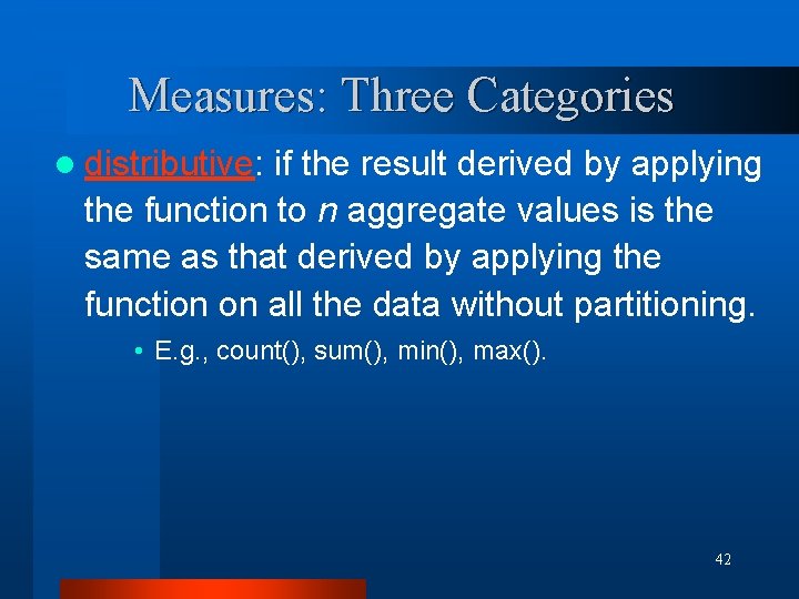
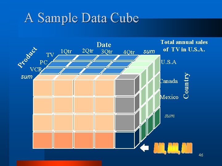
From Tables and Spreadsheets to Data Cubes l A data cube, such as sales, allows data to be modeled and viewed in multiple dimensions – Dimension tables, such as item (item_name, brand, type), or time(day, week, month, quarter, year) – Fact table contains measures (such as dollars_sold) and keys to each of the related dimension tables 24

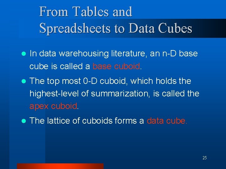
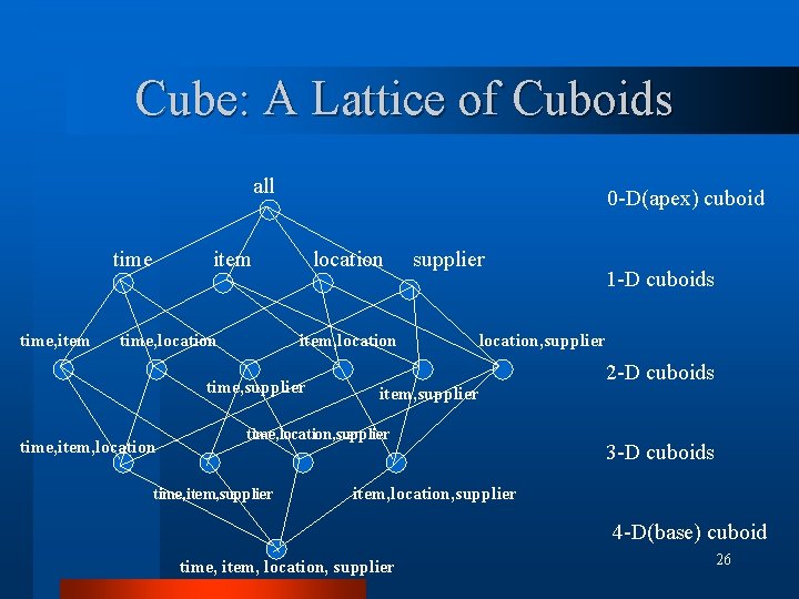
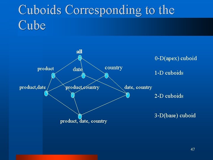
From Tables and Spreadsheets to Data Cubes l In data warehousing literature, an n-D base cube is called a base cuboid. l The top most 0 -D cuboid, which holds the highest-level of summarization, is called the apex cuboid. l The lattice of cuboids forms a data cube. 25

Cube: A Lattice of Cuboids all time, item 0 -D(apex) cuboid item time, location item, location time, supplier time, item, location supplier location, supplier item, supplier time, location, supplier time, item, supplier 1 -D cuboids 2 -D cuboids 3 -D cuboids item, location, supplier 4 -D(base) cuboid time, item, location, supplier 26

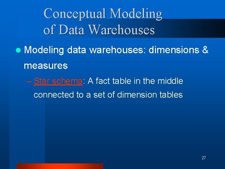
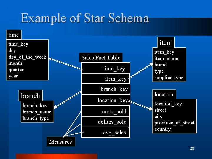
Conceptual Modeling of Data Warehouses l Modeling data warehouses: dimensions & measures – Star schema: A fact table in the middle connected to a set of dimension tables 27

Example of Star Schema time item time_key day_of_the_week month quarter year Sales Fact Table time_key item_key branch_key branch_name branch_type location_key units_sold dollars_sold avg_sales item_key item_name brand type supplier_type location_key street city province_or_street country Measures 28

Conceptual Modeling of Data Warehouses – Snowflake schema: A refinement of star schema where some dimensional hierarchy is normalized into a set of smaller dimension tables, forming a shape similar to snowflake 29

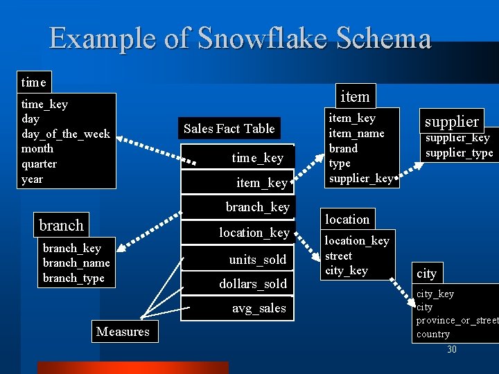
Example of Snowflake Schema time_key day_of_the_week month quarter year item Sales Fact Table time_key item_key branch location_key branch_name branch_type units_sold dollars_sold avg_sales Measures item_key item_name brand type supplier_key supplier_type location_key street city_key city province_or_street country 30

Conceptual Modeling of Data Warehouses – Fact constellations: Multiple fact tables share dimension tables, viewed as a collection of stars, therefore called galaxy schema or fact constellation 31

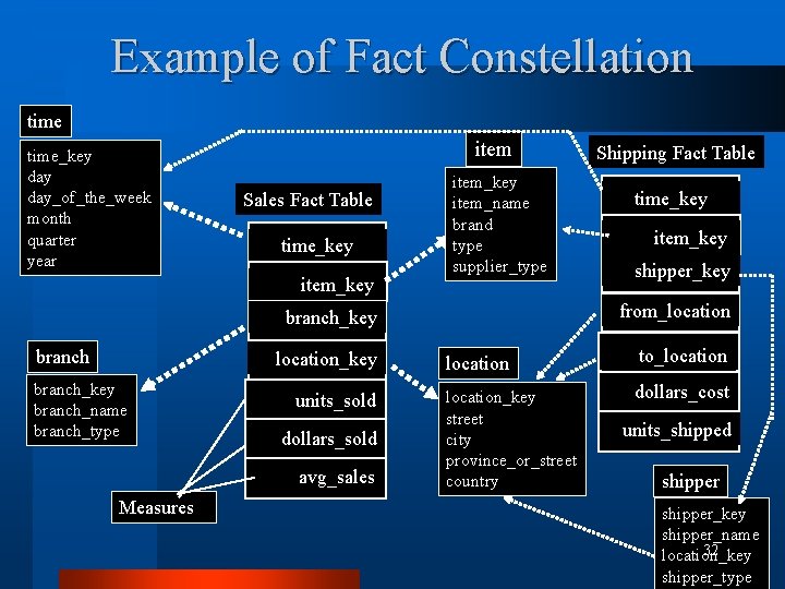
Example of Fact Constellation time_key day_of_the_week month quarter year item Sales Fact Table time_key item_key item_name brand type supplier_type location_key branch_name branch_type units_sold dollars_sold avg_sales Measures time_key item_key shipper_key from_location branch_key branch Shipping Fact Table location to_location_key street city province_or_street country dollars_cost units_shipped shipper_key shipper_name 32 location_key shipper_type

A Data Mining Query Language DMQL 33

Language Primitives l Cube Definition (Fact Table) define cube <cube_name> [<dimension_list>]: <measure_list> l Dimension Definition ( Dimension Table ) define dimension <dimension_name> as (<attribute_or_subdimension_list>) 34

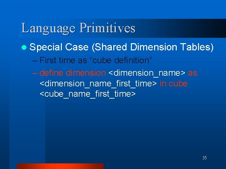
Language Primitives l Special Case (Shared Dimension Tables) – First time as “cube definition” – define dimension <dimension_name> as <dimension_name_first_time> in cube <cube_name_first_time> 35

Defining a Star Schema in DMQL define cube sales_star [time, item, branch, location]: dollars_sold = sum(sales_in_dollars), avg_sales = avg(sales_in_dollars), units_sold = count(*) define dimension time as (time_key, day_of_week, month, quarter, year) 36

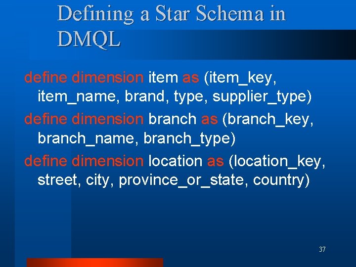
Defining a Star Schema in DMQL define dimension item as (item_key, item_name, brand, type, supplier_type) define dimension branch as (branch_key, branch_name, branch_type) define dimension location as (location_key, street, city, province_or_state, country) 37

Defining a Snowflake Schema in DMQL define cube sales_snowflake [time, item, branch, location]: dollars_sold = sum(sales_in_dollars), avg_sales = avg(sales_in_dollars), units_sold = count(*) define dimension time as (time_key, day_of_week, month, quarter, year) 38

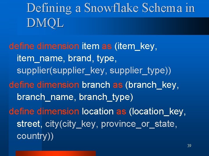
Defining a Snowflake Schema in DMQL define dimension item as (item_key, item_name, brand, type, supplier(supplier_key, supplier_type)) define dimension branch as (branch_key, branch_name, branch_type) define dimension location as (location_key, street, city(city_key, province_or_state, country)) 39

Defining a Fact Constellation in DMQL define cube sales [time, item, branch, location]: dollars_sold = sum(sales_in_dollars), avg_sales = avg(sales_in_dollars), units_sold = count(*) define dimension time as (time_key, day_of_week, month, quarter, year) define dimension item as (item_key, item_name, brand, type, supplier_type) define dimension branch as (branch_key, branch_name, branch_type) define dimension location as (location_key, street, city, province_or_state, country) 40

Defining a Fact Constellation in DMQL define cube shipping [time, item, shipper, from_location, to_location]: dollar_cost = sum(cost_in_dollars), unit_shipped = count(*) define dimension time as time in cube sales define dimension item as item in cube sales define dimension shipper as (shipper_key, shipper_name, location as location in cube sales, shipper_type) define dimension from_location as location in cube sales define dimension to_location as location in cube sales 41

Measures: Three Categories l distributive: if the result derived by applying the function to n aggregate values is the same as that derived by applying the function on all the data without partitioning. • E. g. , count(), sum(), min(), max(). 42

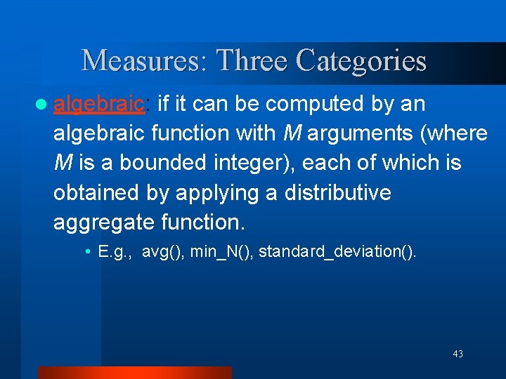
Measures: Three Categories l algebraic: if it can be computed by an algebraic function with M arguments (where M is a bounded integer), each of which is obtained by applying a distributive aggregate function. • E. g. , avg(), min_N(), standard_deviation(). 43

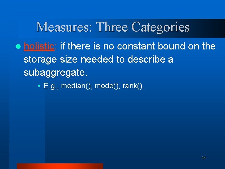
Measures: Three Categories l holistic: if there is no constant bound on the storage size needed to describe a subaggregate. • E. g. , median(), mode(), rank(). 44

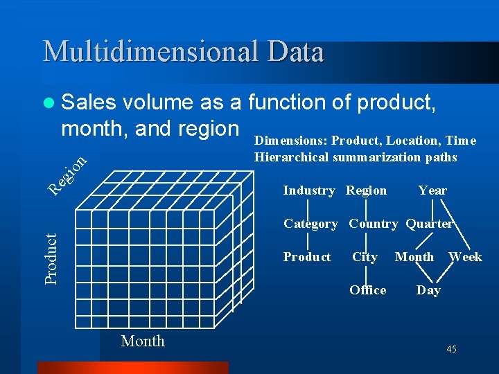
Multidimensional Data l Sales volume as a function of product, month, and region Dimensions: Product, Location, Time gi on Hierarchical summarization paths Re Industry Region Year Product Category Country Quarter Product City Office Month Week Day 45

Pr od TV PC VCR sum 1 Qtr 2 Qtr Date 3 Qtr 4 Qtr Total annual sales sum of TV in U. S. A Canada Mexico Country uc t A Sample Data Cube sum 46

Cuboids Corresponding to the Cube all 0 -D(apex) cuboid product, date country product, country 1 -D cuboids date, country 2 -D cuboids product, date, country 3 -D(base) cuboid 47

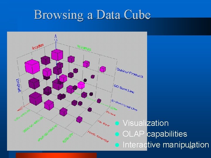
Browsing a Data Cube Visualization l OLAP capabilities l Interactive manipulation 48 l

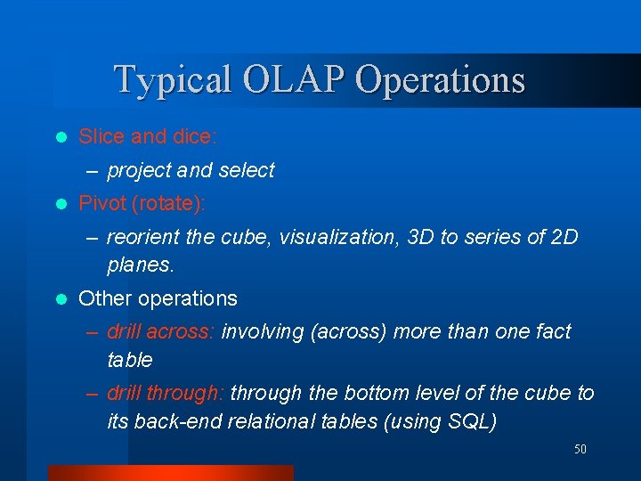
Typical OLAP Operations l Roll up (drill-up): summarize data – by climbing up hierarchy or by dimension reduction l Drill down (roll down): reverse of roll-up – from higher level summary to lower level summary or detailed data, or introducing new dimensions 49

Typical OLAP Operations l Slice and dice: – project and select l Pivot (rotate): – reorient the cube, visualization, 3 D to series of 2 D planes. l Other operations – drill across: involving (across) more than one fact table – drill through: through the bottom level of the cube to its back-end relational tables (using SQL) 50

Data Warehouse Architecture 51

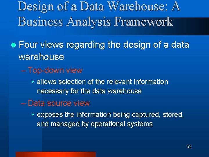
Design of a Data Warehouse: A Business Analysis Framework l Four views regarding the design of a data warehouse – Top-down view • allows selection of the relevant information necessary for the data warehouse – Data source view • exposes the information being captured, stored, and managed by operational systems 52

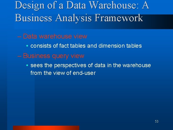
Design of a Data Warehouse: A Business Analysis Framework – Data warehouse view • consists of fact tables and dimension tables – Business query view • sees the perspectives of data in the warehouse from the view of end-user 53

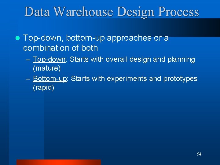
Data Warehouse Design Process l Top-down, bottom-up approaches or a combination of both – Top-down: Starts with overall design and planning (mature) – Bottom-up: Starts with experiments and prototypes (rapid) 54

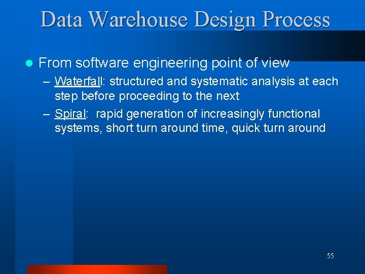
Data Warehouse Design Process l From software engineering point of view – Waterfall: structured and systematic analysis at each step before proceeding to the next – Spiral: rapid generation of increasingly functional systems, short turn around time, quick turn around 55

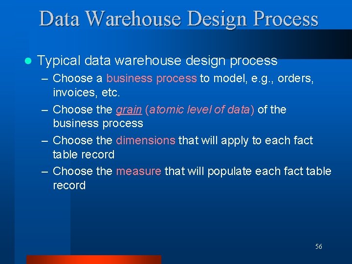
Data Warehouse Design Process l Typical data warehouse design process – Choose a business process to model, e. g. , orders, invoices, etc. – Choose the grain (atomic level of data) of the business process – Choose the dimensions that will apply to each fact table record – Choose the measure that will populate each fact table record 56

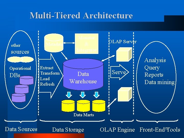
Multi-Tiered Architecture other Metadata sources Operational DBs Extract Transform Load Refresh Monitor & Integrator Data Warehouse OLAP Server Serve Analysis Query Reports Data mining Data Marts Data Sources Data Storage OLAP Engine Front-End 57 Tools

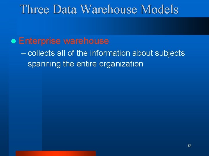
Three Data Warehouse Models l Enterprise warehouse – collects all of the information about subjects spanning the entire organization 58

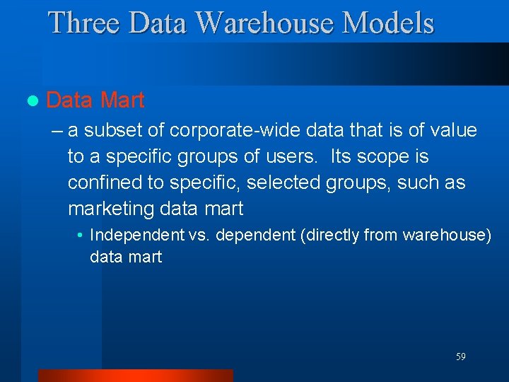
Three Data Warehouse Models l Data Mart – a subset of corporate-wide data that is of value to a specific groups of users. Its scope is confined to specific, selected groups, such as marketing data mart • Independent vs. dependent (directly from warehouse) data mart 59

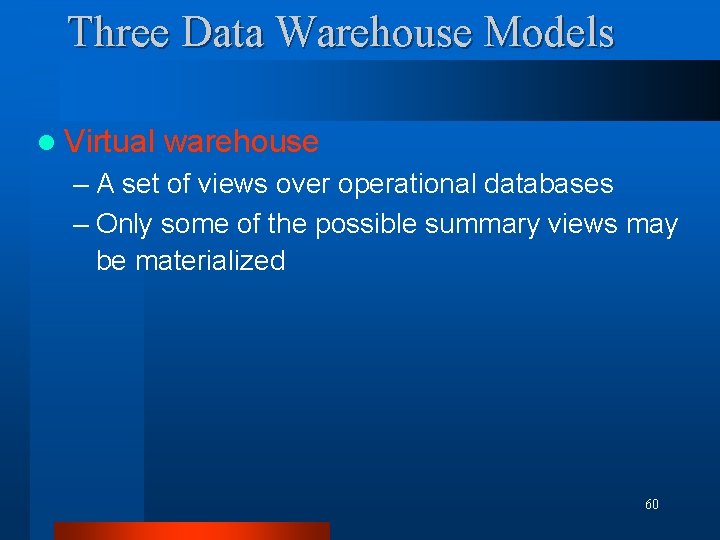
Three Data Warehouse Models l Virtual warehouse – A set of views over operational databases – Only some of the possible summary views may be materialized 60

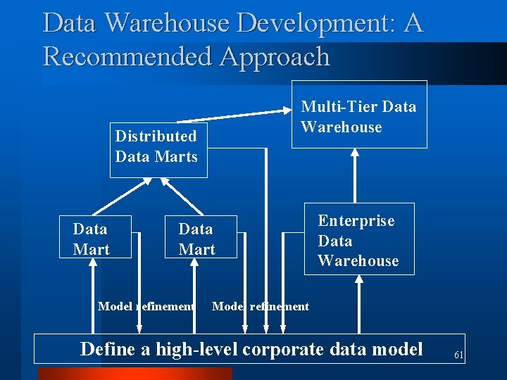
Data Warehouse Development: A Recommended Approach Multi-Tier Data Warehouse Distributed Data Marts Data Mart Model refinement Enterprise Data Warehouse Model refinement Define a high-level corporate data model 61

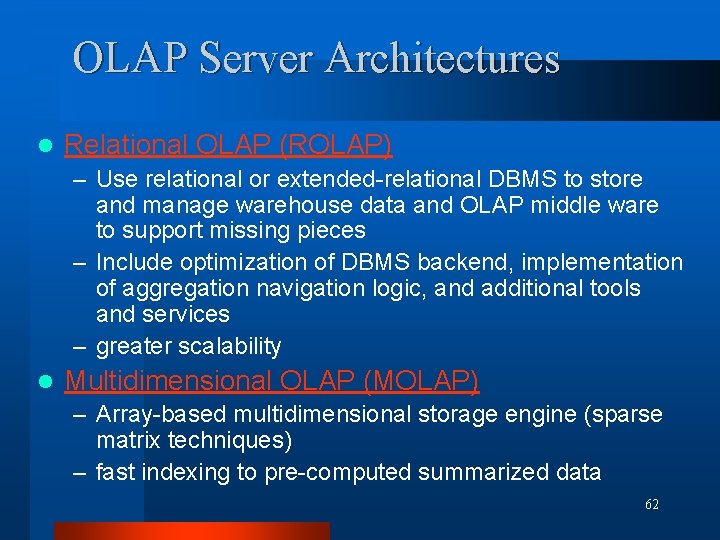
OLAP Server Architectures l Relational OLAP (ROLAP) – Use relational or extended-relational DBMS to store and manage warehouse data and OLAP middle ware to support missing pieces – Include optimization of DBMS backend, implementation of aggregation navigation logic, and additional tools and services – greater scalability l Multidimensional OLAP (MOLAP) – Array-based multidimensional storage engine (sparse matrix techniques) – fast indexing to pre-computed summarized data 62

OLAP Server Architectures l Hybrid OLAP (HOLAP) – User flexibility, e. g. , low level: relational, high-level: array l Specialized SQL servers – specialized support for SQL queries over star/snowflake schemas 63

Data Warehouse Implementation 64

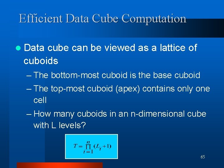
Efficient Data Cube Computation l Data cube can be viewed as a lattice of cuboids – The bottom-most cuboid is the base cuboid – The top-most cuboid (apex) contains only one cell – How many cuboids in an n-dimensional cube with L levels? 65

Efficient Data Cube Computation l Materialization of data cube – Materialize every (cuboid) (full materialization), none (no materialization), or some (partial materialization) – Selection of which cuboids to materialize • Based on size, sharing, access frequency, etc. 66

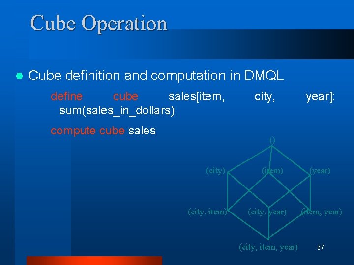
Cube Operation l Cube definition and computation in DMQL define cube sales[item, sum(sales_in_dollars) compute cube sales city, year]: () (city, item) (year) (city, year) (item, year) (city, item, year) 67

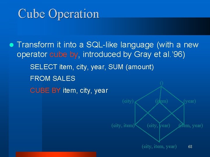
Cube Operation l Transform it into a SQL-like language (with a new operator cube by, introduced by Gray et al. ’ 96) SELECT item, city, year, SUM (amount) FROM SALES () CUBE BY item, city, year (city) (city, item) (year) (city, year) (item, year) (city, item, year) 68

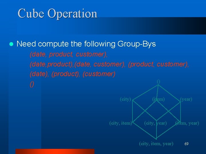
Cube Operation l Need compute the following Group-Bys (date, product, customer), (date, product), (date, customer), (product, customer), (date), (product), (customer) () () (city, item) (year) (city, year) (item, year) (city, item, year) 69

Cube Computation: ROLAP-Based Method l Efficient cube computation methods – ROLAP-based cubing algorithms (Agarwal et al’ 96) – Array-based cubing algorithm (Zhao et al’ 97) – Bottom-up computation method (Bayer & Ramarkrishnan’ 99) 70

Cube Computation: ROLAP-Based Method l ROLAP-based cubing algorithms – Sorting, hashing, and grouping operations are applied to the dimension attributes in order to reorder and cluster related tuples – Grouping is performed on some subaggregates as a “partial grouping step” – Aggregates may be computed from previously computed aggregates, rather than from the base fact table 71

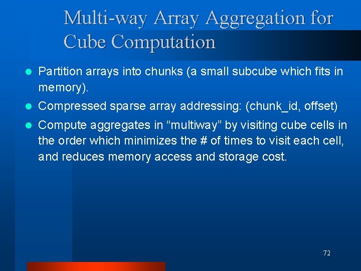
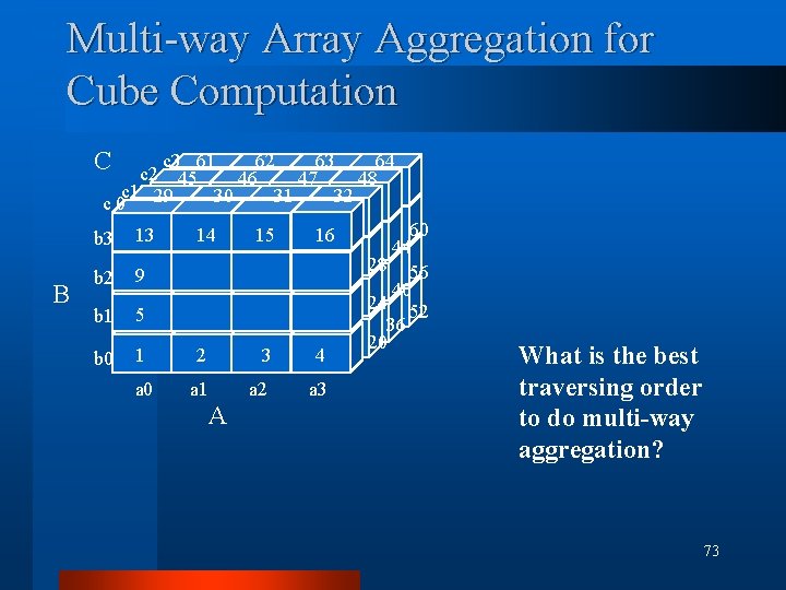
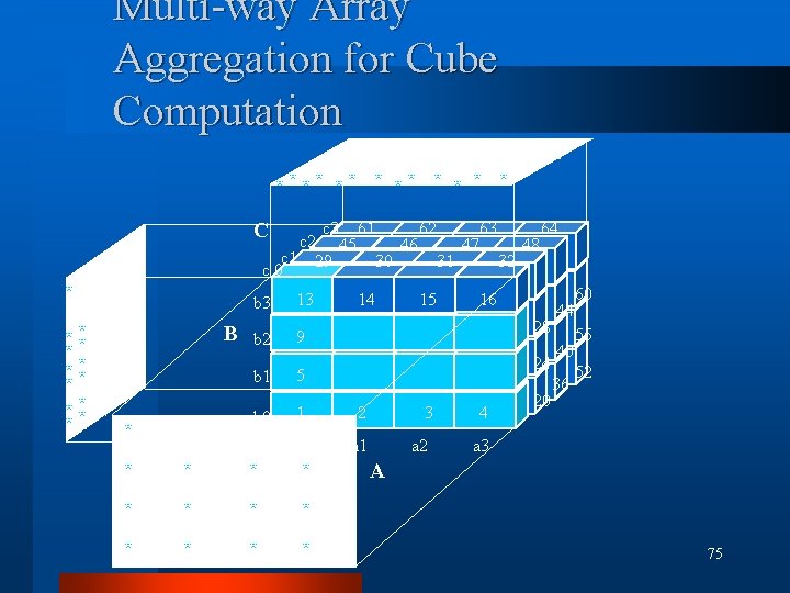
Multi-way Array Aggregation for Cube Computation l Partition arrays into chunks (a small subcube which fits in memory). l Compressed sparse array addressing: (chunk_id, offset) l Compute aggregates in “multiway” by visiting cube cells in the order which minimizes the # of times to visit each cell, and reduces memory access and storage cost. 72

Multi-way Array Aggregation for Cube Computation C c 3 61 62 63 64 c 2 45 46 47 48 c 1 29 30 31 32 c 0 B b 3 B 13 b 2 9 b 1 5 b 0 14 15 16 1 2 3 4 a 0 a 1 a 2 a 3 A 60 44 28 56 40 24 52 36 20 What is the best traversing order to do multi-way aggregation? 73

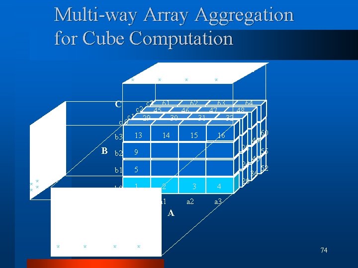
Multi-way Array Aggregation for Cube Computation C c 3 61 62 63 64 c 2 45 46 47 48 c 1 29 30 31 32 c 0 b 3 B b 2 B 13 14 15 16 28 9 24 b 1 5 b 0 1 2 3 4 a 0 a 1 a 2 a 3 20 44 40 36 60 56 52 A 74

Multi-way Array Aggregation for Cube Computation C c 3 61 62 63 64 c 2 45 46 47 48 c 1 29 30 31 32 c 0 b 3 B b 2 B 13 14 15 16 28 9 24 b 1 5 b 0 1 2 3 4 a 0 a 1 a 2 a 3 20 44 40 36 60 56 52 A 75

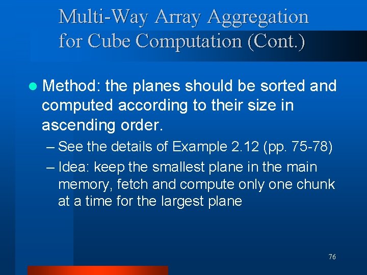
Multi-Way Array Aggregation for Cube Computation (Cont. ) l Method: the planes should be sorted and computed according to their size in ascending order. – See the details of Example 2. 12 (pp. 75 -78) – Idea: keep the smallest plane in the main memory, fetch and compute only one chunk at a time for the largest plane 76

Multi-Way Array Aggregation for Cube Computation (Cont. ) l Limitation of the method: computing well only for a small number of dimensions – If there a large number of dimensions, “bottom-up computation” and iceberg cube computation methods can be explored 77

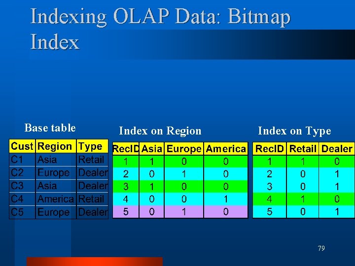
Indexing OLAP Data: Bitmap Index l l l Index on a particular column Each value in the column has a bit vector: bitop is fast The length of the bit vector: # of records in the base table The i-th bit is set if the i-th row of the base table has the value for the indexed column not suitable for high cardinality domains 78

Indexing OLAP Data: Bitmap Index Base table Index on Region Index on Type 79

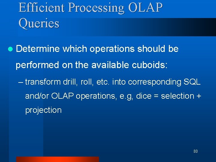
Efficient Processing OLAP Queries l Determine which operations should be performed on the available cuboids: – transform drill, roll, etc. into corresponding SQL and/or OLAP operations, e. g, dice = selection + projection 80

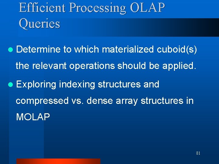
Efficient Processing OLAP Queries l Determine to which materialized cuboid(s) the relevant operations should be applied. l Exploring indexing structures and compressed vs. dense array structures in MOLAP 81

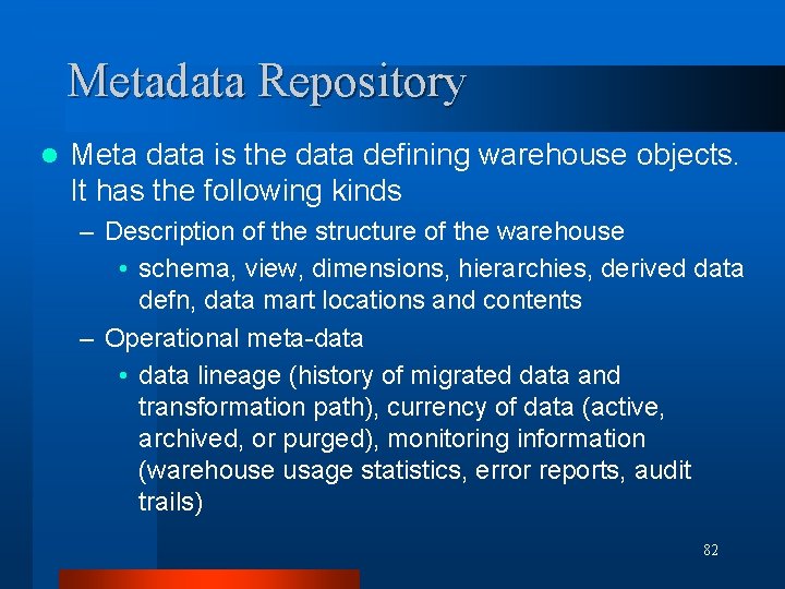
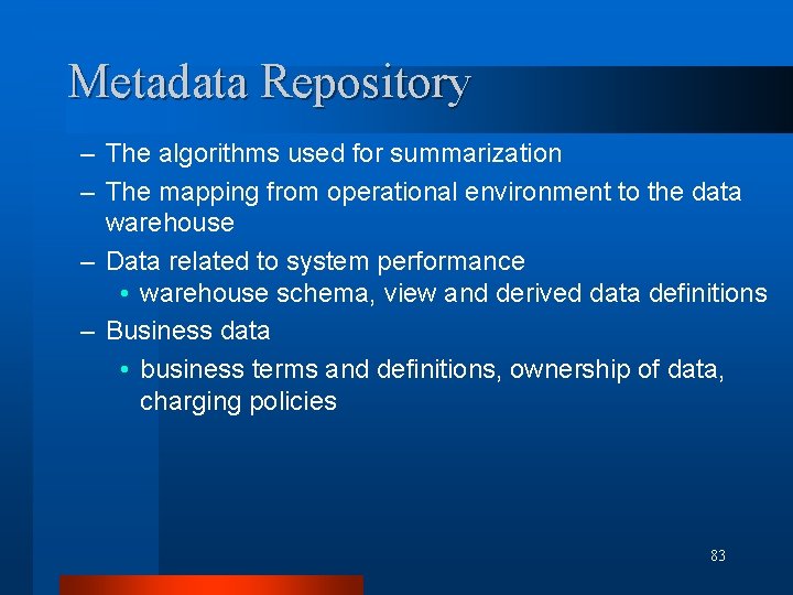
Metadata Repository l Meta data is the data defining warehouse objects. It has the following kinds – Description of the structure of the warehouse • schema, view, dimensions, hierarchies, derived data defn, data mart locations and contents – Operational meta-data • data lineage (history of migrated data and transformation path), currency of data (active, archived, or purged), monitoring information (warehouse usage statistics, error reports, audit trails) 82

Metadata Repository – The algorithms used for summarization – The mapping from operational environment to the data warehouse – Data related to system performance • warehouse schema, view and derived data definitions – Business data • business terms and definitions, ownership of data, charging policies 83

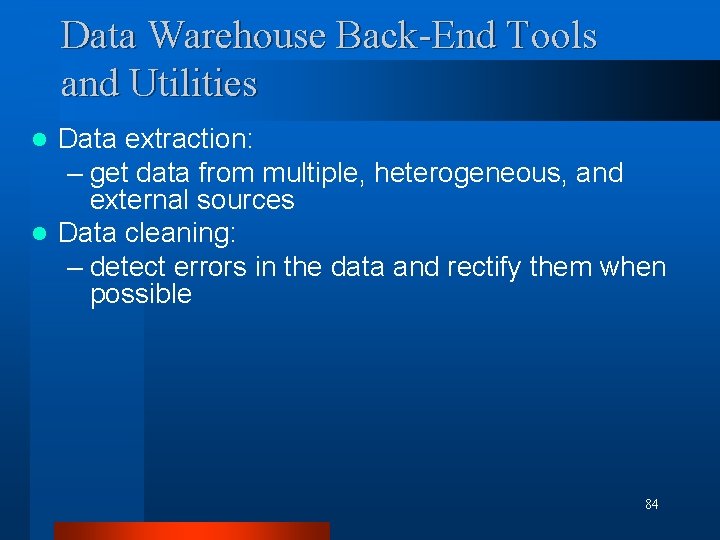
Data Warehouse Back-End Tools and Utilities Data extraction: – get data from multiple, heterogeneous, and external sources l Data cleaning: – detect errors in the data and rectify them when possible l 84

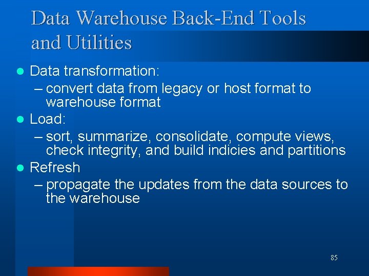
Data Warehouse Back-End Tools and Utilities Data transformation: – convert data from legacy or host format to warehouse format l Load: – sort, summarize, consolidate, compute views, check integrity, and build indicies and partitions l Refresh – propagate the updates from the data sources to the warehouse l 85

Further Development of Data Cube Technology 86

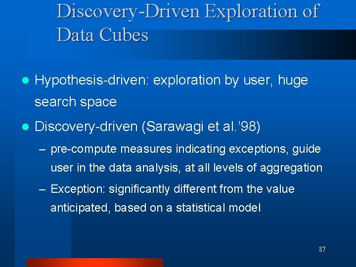
Discovery-Driven Exploration of Data Cubes l Hypothesis-driven: exploration by user, huge search space l Discovery-driven (Sarawagi et al. ’ 98) – pre-compute measures indicating exceptions, guide user in the data analysis, at all levels of aggregation – Exception: significantly different from the value anticipated, based on a statistical model 87

From Data Warehousing to Data Mining 88

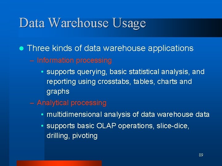
Data Warehouse Usage l Three kinds of data warehouse applications – Information processing • supports querying, basic statistical analysis, and reporting using crosstabs, tables, charts and graphs – Analytical processing • multidimensional analysis of data warehouse data • supports basic OLAP operations, slice-dice, drilling, pivoting 89

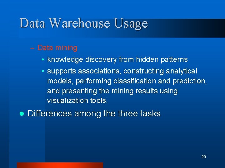
Data Warehouse Usage – Data mining • knowledge discovery from hidden patterns • supports associations, constructing analytical models, performing classification and prediction, and presenting the mining results using visualization tools. l Differences among the three tasks 90

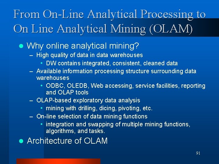
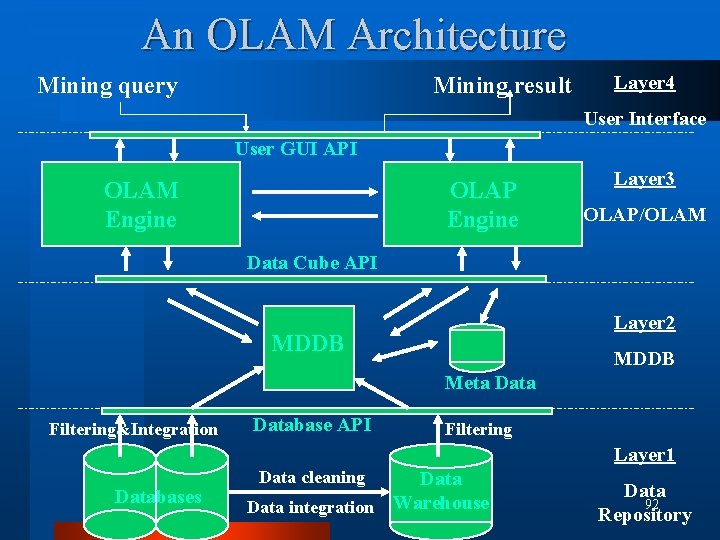
From On-Line Analytical Processing to On Line Analytical Mining (OLAM) l Why online analytical mining? – High quality of data in data warehouses • DW contains integrated, consistent, cleaned data – Available information processing structure surrounding data warehouses • ODBC, OLEDB, Web accessing, service facilities, reporting and OLAP tools – OLAP-based exploratory data analysis • mining with drilling, dicing, pivoting, etc. – On-line selection of data mining functions • integration and swapping of multiple mining functions, algorithms, and tasks. l Architecture of OLAM 91

An OLAM Architecture Mining query Mining result Layer 4 User Interface User GUI API OLAM Engine OLAP Engine Layer 3 OLAP/OLAM Data Cube API Layer 2 MDDB Meta Data Filtering&Integration Database API Filtering Layer 1 Databases Data cleaning Data integration Warehouse Data 92 Repository

Data Mining 93

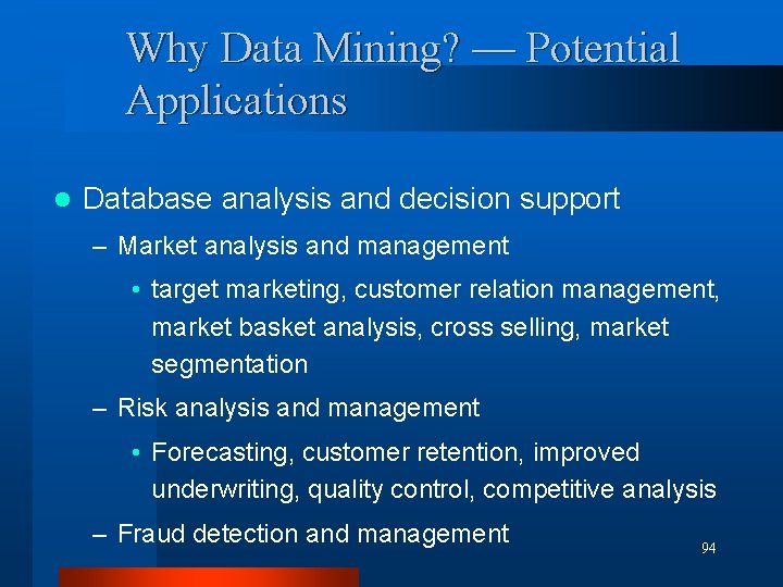
Why Data Mining? — Potential Applications l Database analysis and decision support – Market analysis and management • target marketing, customer relation management, market basket analysis, cross selling, market segmentation – Risk analysis and management • Forecasting, customer retention, improved underwriting, quality control, competitive analysis – Fraud detection and management 94

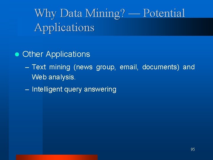
Why Data Mining? — Potential Applications l Other Applications – Text mining (news group, email, documents) and Web analysis. – Intelligent query answering 95

Material taken from http: //www. cs. sfu. ca/~han Tiempo para descansar !!! 96