Introduction to Data Mining and Classification F Michael

Introduction to Data Mining and Classification F. Michael Speed, Ph. D. Analytical Consultant SAS Global Academic Program Copyright © 2010, SAS Institute Inc. All rights reserved.

Objectives • State one of the major principles underlying data mining • Give a high level overview of three classification procedures 2

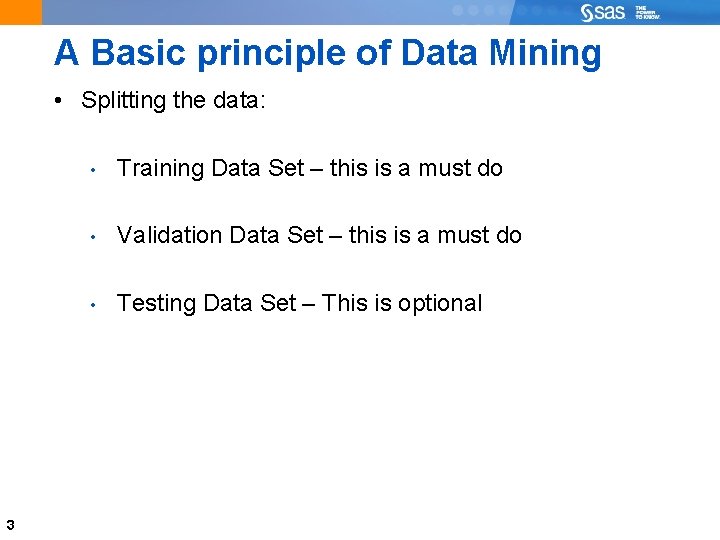
A Basic principle of Data Mining • Splitting the data: 3 • Training Data Set – this is a must do • Validation Data Set – this is a must do • Testing Data Set – This is optional

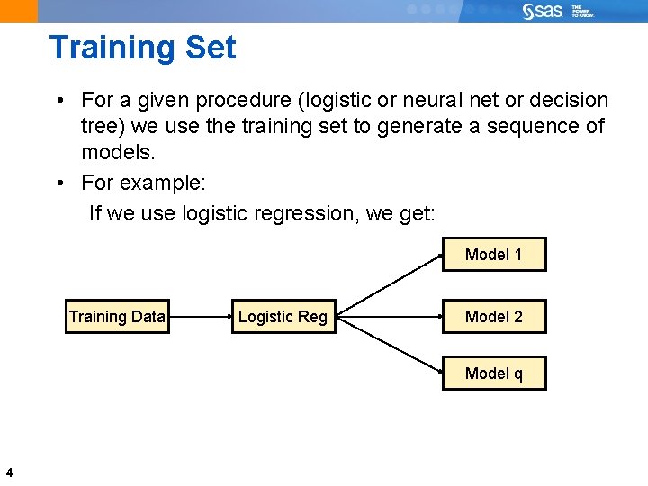
Training Set • For a given procedure (logistic or neural net or decision tree) we use the training set to generate a sequence of models. • For example: If we use logistic regression, we get: Model 1 Training Data Logistic Reg Model 2 Model q 4

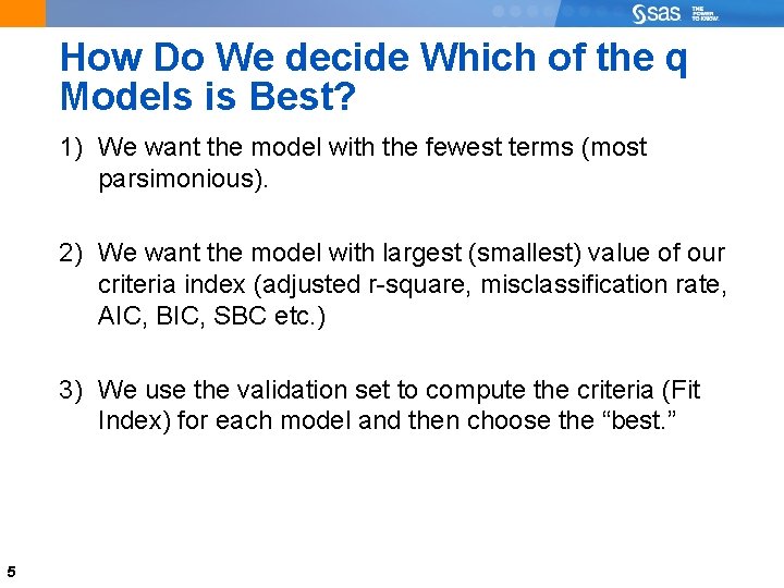
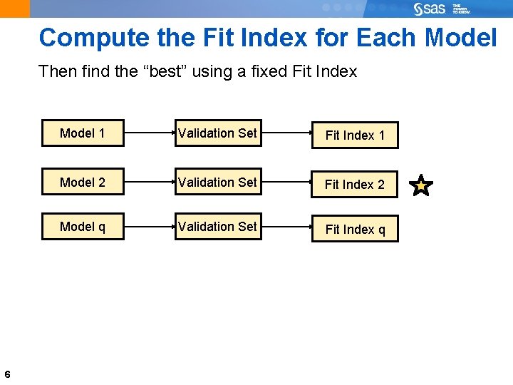
How Do We decide Which of the q Models is Best? 1) We want the model with the fewest terms (most parsimonious). 2) We want the model with largest (smallest) value of our criteria index (adjusted r-square, misclassification rate, AIC, BIC, SBC etc. ) 3) We use the validation set to compute the criteria (Fit Index) for each model and then choose the “best. ” 5

Compute the Fit Index for Each Model Then find the “best” using a fixed Fit Index 6 Model 1 Validation Set Fit Index 1 Model 2 Validation Set Fit Index 2 Model q Validation Set Fit Index q

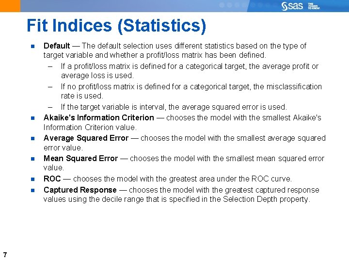
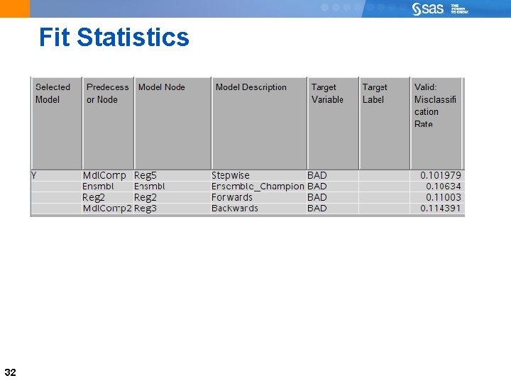
Fit Indices (Statistics) 7 Default — The default selection uses different statistics based on the type of target variable and whether a profit/loss matrix has been defined. – If a profit/loss matrix is defined for a categorical target, the average profit or average loss is used. – If no profit/loss matrix is defined for a categorical target, the misclassification rate is used. – If the target variable is interval, the average squared error is used. Akaike's Information Criterion — chooses the model with the smallest Akaike's Information Criterion value. Average Squared Error — chooses the model with the smallest average squared error value. Mean Squared Error — chooses the model with the smallest mean squared error value. ROC — chooses the model with the greatest area under the ROC curve. Captured Response — chooses the model with the greatest captured response values using the decile range that is specified in the Selection Depth property.

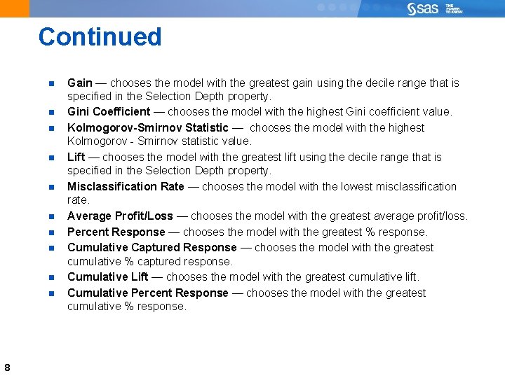
Continued 8 Gain — chooses the model with the greatest gain using the decile range that is specified in the Selection Depth property. Gini Coefficient — chooses the model with the highest Gini coefficient value. Kolmogorov-Smirnov Statistic — chooses the model with the highest Kolmogorov - Smirnov statistic value. Lift — chooses the model with the greatest lift using the decile range that is specified in the Selection Depth property. Misclassification Rate — chooses the model with the lowest misclassification rate. Average Profit/Loss — chooses the model with the greatest average profit/loss. Percent Response — chooses the model with the greatest % response. Cumulative Captured Response — chooses the model with the greatest cumulative % captured response. Cumulative Lift — chooses the model with the greatest cumulative lift. Cumulative Percent Response — chooses the model with the greatest cumulative % response.

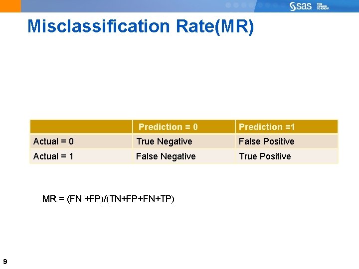
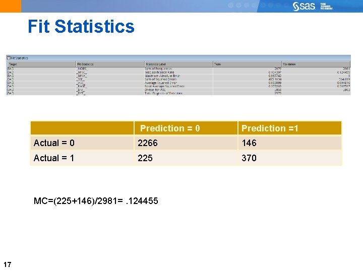
Misclassification Rate(MR) Prediction = 0 Prediction =1 Actual = 0 True Negative False Positive Actual = 1 False Negative True Positive MR = (FN +FP)/(TN+FP+FN+TP) 9

Equity Data Set. • The variable BAD = 1 if the borrower is a bad credit risk and = 0 if not. • We want to build a model to predict if a person is a bad credit risk • Other Variables: Job, YOJ, Loan, Debt. Inc • • 10 Mortdue - How much they need to pay on their mortgage Value - Assessed valuation Derog - Number of Derogatory Reports Deliniq - Number of Delinquent Trade Lines Clage - Age of Oldest Trade Line Ninq - Number of recent credit inquiries. Clno - Number of trade lines

Three Procedures Decision Tree Regression (Logistic) Neural Network 11

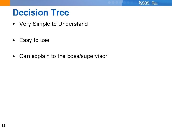
Decision Tree • Very Simple to Understand • Easy to use • Can explain to the boss/supervisor 12

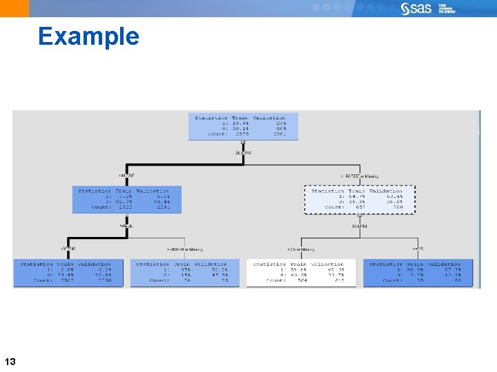
Example 13

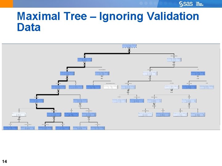
Maximal Tree – Ignoring Validation Data 14

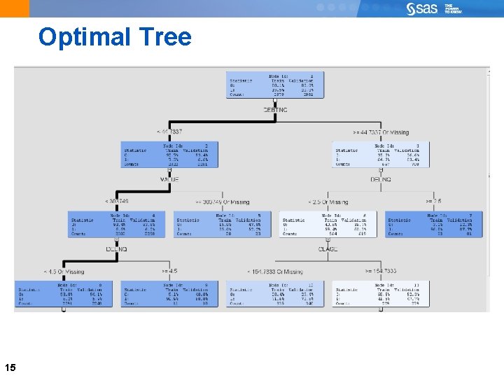
Optimal Tree 15

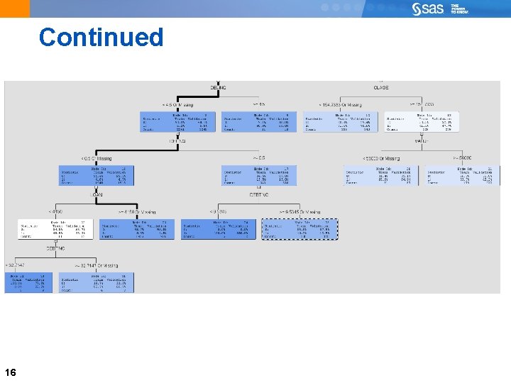
Continued 16

Fit Statistics Prediction = 0 Prediction =1 Actual = 0 2266 146 Actual = 1 225 370 MC=(225+146)/2981=. 124455 17

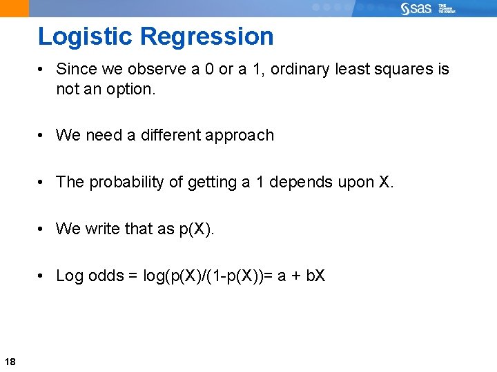
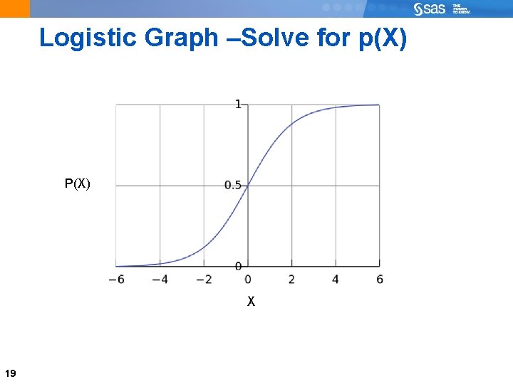
Logistic Regression • Since we observe a 0 or a 1, ordinary least squares is not an option. • We need a different approach • The probability of getting a 1 depends upon X. • We write that as p(X). • Log odds = log(p(X)/(1 -p(X))= a + b. X 18

Logistic Graph –Solve for p(X) P(X) X 19

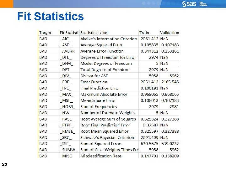
Fit Statistics 20

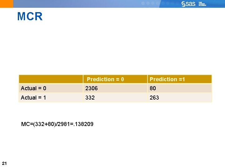
MCR Prediction = 0 Prediction =1 Actual = 0 2306 80 Actual = 1 332 263 MC=(332+80)/2981=. 138209 21

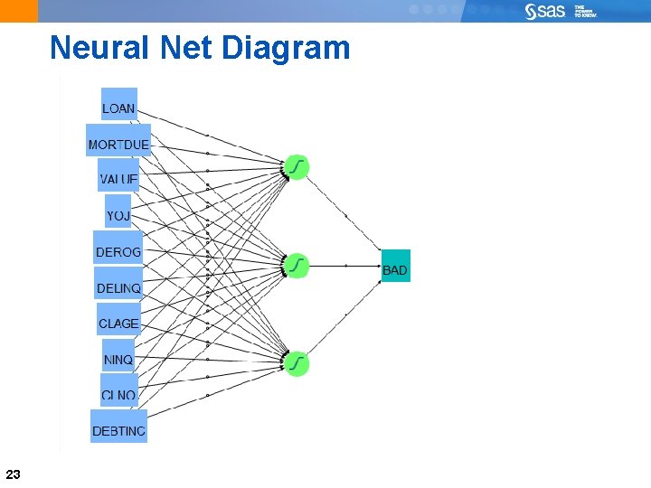
Neural Net Very Complex Mathematical Equations Interpretations of the meaning of the input variables are not possible with final model Often a good prediction of the response. 22

Neural Net Diagram 23

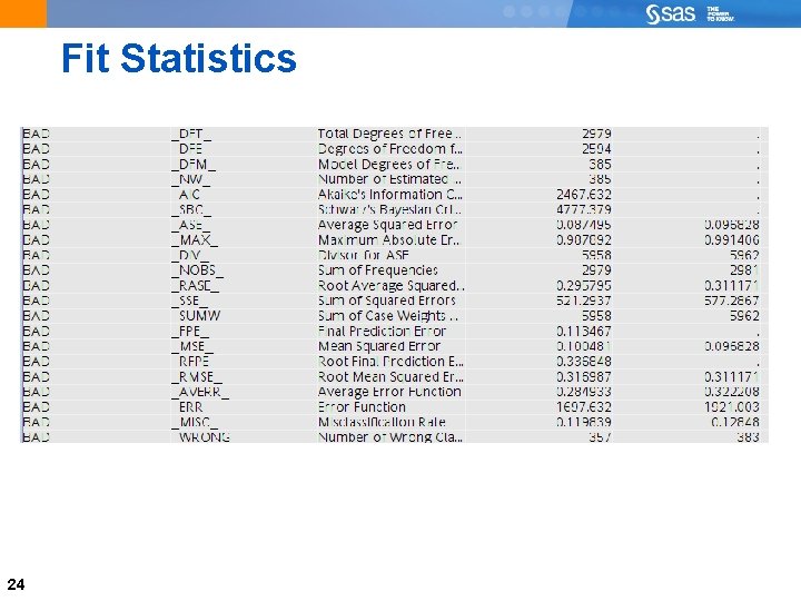
Fit Statistics 24

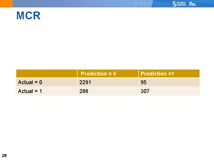
MCR 25 Prediction = 0 Prediction =1 Actual = 0 2291 95 Actual = 1 288 307

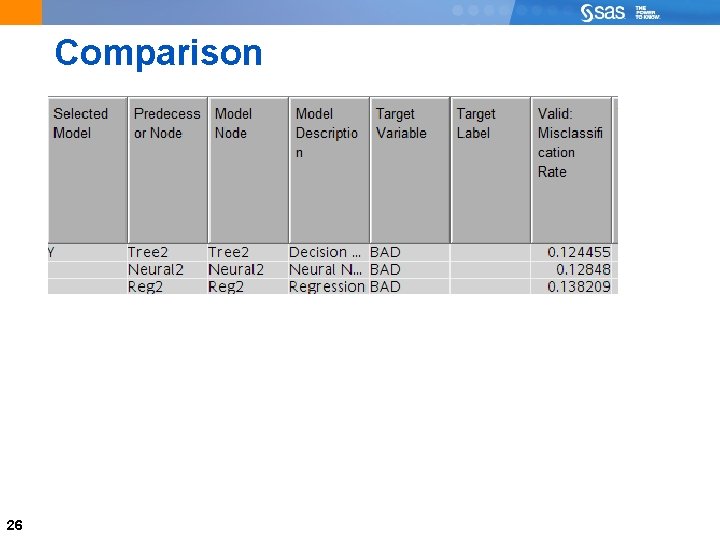
Comparison 26

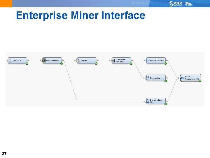
Enterprise Miner Interface 27

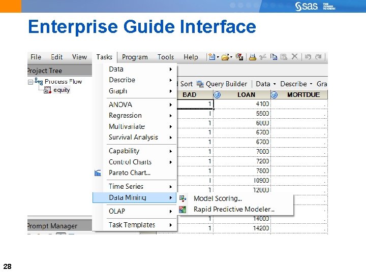
Enterprise Guide Interface 28

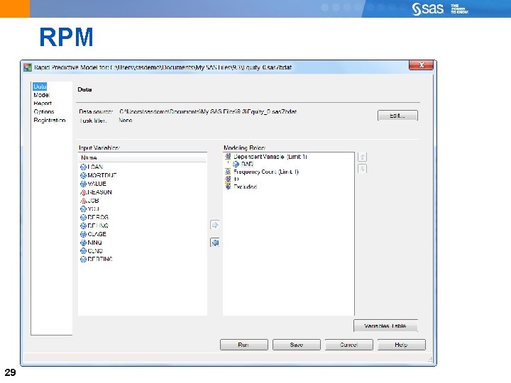
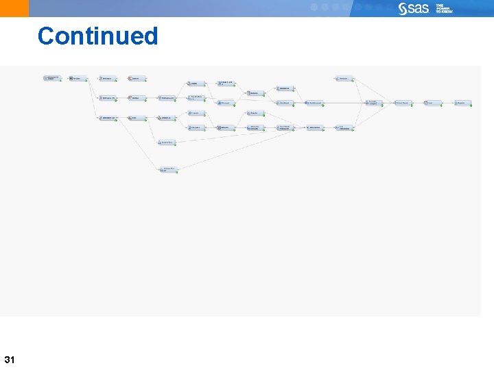
RPM 29

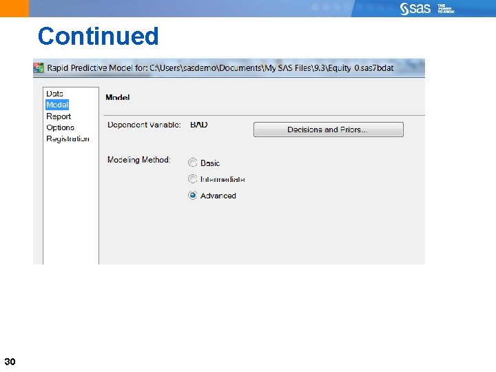
Continued 30

Continued 31

Fit Statistics 32

Summary 1) Divide your data into training and validation 2) We looked at trees, logistic regression and neural nets 3) We also looked at RPM 33

Q&A 34