Introduction to Data Analysis The Role of Data

Introduction to Data Analysis – The Role of Data Analysis in Test and Product Engineering – The process by which we examine test results and draw conclusions from them. » Evaluate DUT design weaknesses, » Identify test repeatability and correlation problems, » Improve test efficiency, » Expose test program bugs » Set test limits » Identify weak production lots (outlier lots) » Optimize wafer fab process 1

Introduction to Data Analysis – The Role of Data Analysis in Test and Product Engineering – Many data analysis tools are designed to help visualize and improve the silicon and assembly fabrication process itself. – The fabrication processes can be improved through statistical data analysis of production test results. – A methodology called statistical process control (SPC) formalizes the steps by which this improvement is achieved. 2

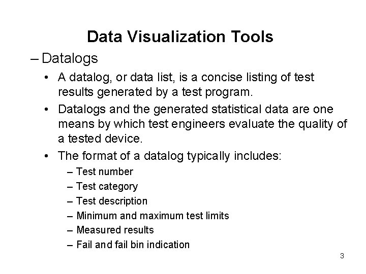
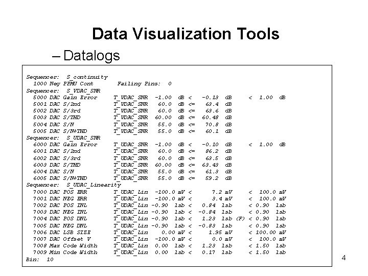
Data Visualization Tools – Datalogs • A datalog, or data list, is a concise listing of test results generated by a test program. • Datalogs and the generated statistical data are one means by which test engineers evaluate the quality of a tested device. • The format of a datalog typically includes: – – – Test number Test category Test description Minimum and maximum test limits Measured results Fail and fail bin indication 3

Data Visualization Tools – Datalogs Sequencer: 1000 Neg Sequencer: 5000 DAC 5001 DAC 5002 DAC 5003 DAC 5004 DAC 5005 DAC Sequencer: 6000 DAC 6001 DAC 6002 DAC 6003 DAC 6004 DAC 6005 DAC Sequencer: 7000 DAC 7001 DAC 7002 DAC 7003 DAC 7004 DAC 7005 DAC 7006 DAC 7007 DAC 7008 Max 7009 Min Bin: 10 S_continuity PPMU Cont Failing Pins: 0 S_VDAC_SNR Gain Error T_VDAC_SNR -1. 00 d. B S/2 nd T_VDAC_SNR 60. 0 d. B S/3 rd T_VDAC_SNR 60. 0 d. B S/THD T_VDAC_SNR 60. 00 d. B S/N T_VDAC_SNR 55. 0 d. B S/N+THD T_VDAC_SNR 55. 0 d. B S_UDAC_SNR Gain Error T_UDAC_SNR -1. 00 d. B S/2 nd T_UDAC_SNR 60. 0 d. B S/3 rd T_UDAC_SNR 60. 0 d. B S/THD T_UDAC_SNR 60. 00 d. B S/N T_UDAC_SNR 55. 0 d. B S/N+THD T_UDAC_SNR 55. 0 d. B S_UDAC_Linearity POS ERR T_UDAC_Lin -100. 0 m. V NEG ERR T_UDAC_Lin -100. 0 m. V POS INL T_UDAC_Lin -0. 90 lsb NEG INL T_UDAC_Lin -0. 90 lsb POS DNL T_UDAC_Lin -0. 90 lsb NEG DNL T_UDAC_Lin -0. 90 lsb LSB SIZE T_UDAC_Lin 0. 00 m. V Offset V T_UDAC_Lin -100. 0 m. V Code Width T_UDAC_Lin 0. 00 lsb < <= <= <= -0. 13 63. 4 63. 6 60. 48 70. 8 60. 1 d. B d. B < 1. 00 d. B < <= <= <= -0. 10 86. 2 63. 5 63. 43 61. 3 59. 2 d. B d. B < 1. 00 d. B < < < < < 7. 2 m. V < 100. 0 m. V 3. 4 m. V < 100. 0 m. V 0. 84 lsb < 0. 90 lsb -0. 84 lsb < 0. 90 lsb 1. 23 lsb (F) < 0. 90 lsb -0. 83 lsb < 0. 90 lsb 1. 95 m. V < 100. 00 m. V 0. 0 m. V < 100. 0 m. V 1. 23 lsb < 1. 50 lsb 0. 17 lsb < 1. 50 lsb 4

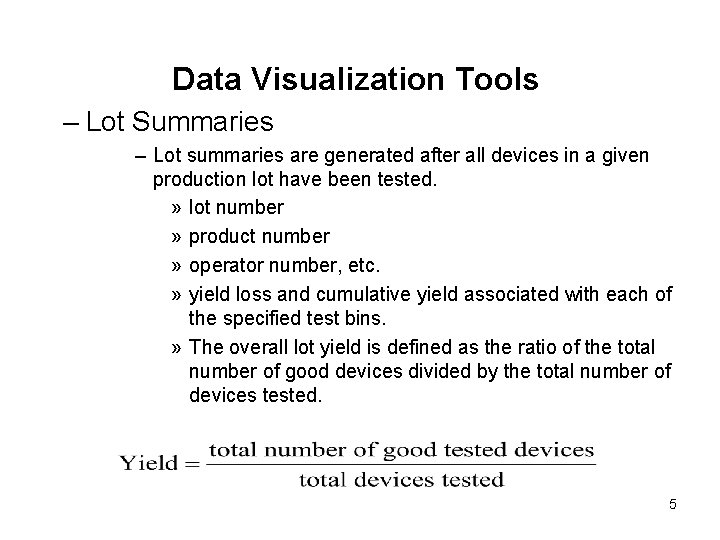
Data Visualization Tools – Lot Summaries – Lot summaries are generated after all devices in a given production lot have been tested. » lot number » product number » operator number, etc. » yield loss and cumulative yield associated with each of the specified test bins. » The overall lot yield is defined as the ratio of the total number of good devices divided by the total number of devices tested. 5

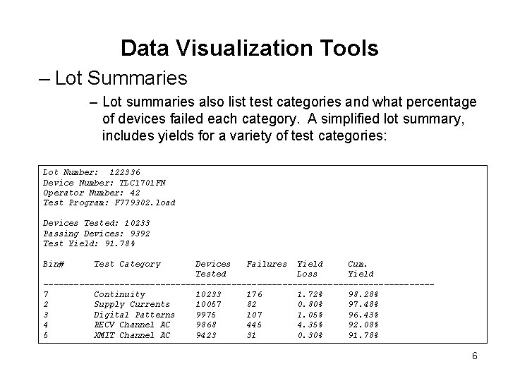
Data Visualization Tools – Lot Summaries – Lot summaries also list test categories and what percentage of devices failed each category. A simplified lot summary, includes yields for a variety of test categories: Lot Number: 122336 Device Number: TLC 1701 FN Operator Number: 42 Test Program: F 779302. load Devices Tested: 10233 Passing Devices: 9392 Test Yield: 91. 78% Bin# Test Category Devices Failures Yield Cum. Tested Loss Yield --------------------------------------7 Continuity 10233 176 1. 72% 98. 28% 2 Supply Currents 10057 82 0. 80% 97. 48% 3 Digital Patterns 9975 107 1. 05% 96. 43% 4 RECV Channel AC 9868 445 4. 35% 92. 08% 5 XMIT Channel AC 9423 31 0. 30% 91. 78% 6

Data Visualization Tools – Lot Summaries – Since the test program halts after the first DUT failure, the earlier tests will tend to cause more yield loss than later ones, simply because fewer DUTs proceed to the later tests. The earlier failures mask any failures that would have occurred in later tests. – The overall production throughput can be optimized by moving the more commonly failed tests toward the beginning of the test program. Average test time might be reduced since no test time is wasted for consecutive failing tests; for multisite test solution this impact might be reduced. – When rearranging test programs based on yield loss, we also have to consider the test time that each test consumes. For example, the RECV channel tests may take 800 milliseconds, while the digital pattern tests only takes 50 milliseconds. The digital pattern test is more efficient at identifying failing DUTs 7 since it takes so little test time.

HW: Assume you have N parts that needs to go through B test bins. Each has test time Ti, i=1, …, B. The probability of fail is Pi. Suppose each test bin is independent of each other. • Derive the order of test so that the expected total test time is minimized. • In this optimized test sequence, obtain the expected yield of each test bin and the expected overall yield. • After you are done testing all N parts, suppose the actual # of fails in each test bin is Fi. Compute the actual yield of each test bin and the actual overall yield. • With actual fail information, how would you update the probabilities?

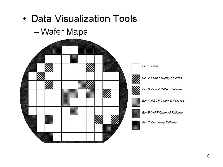
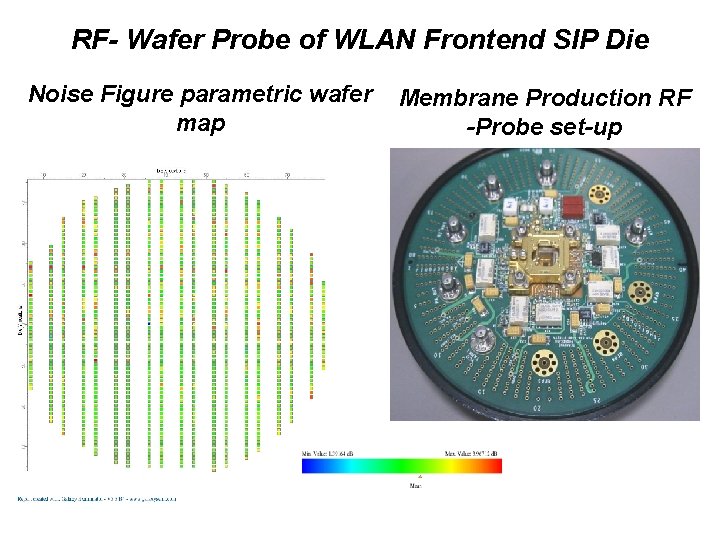
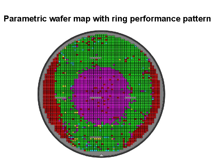
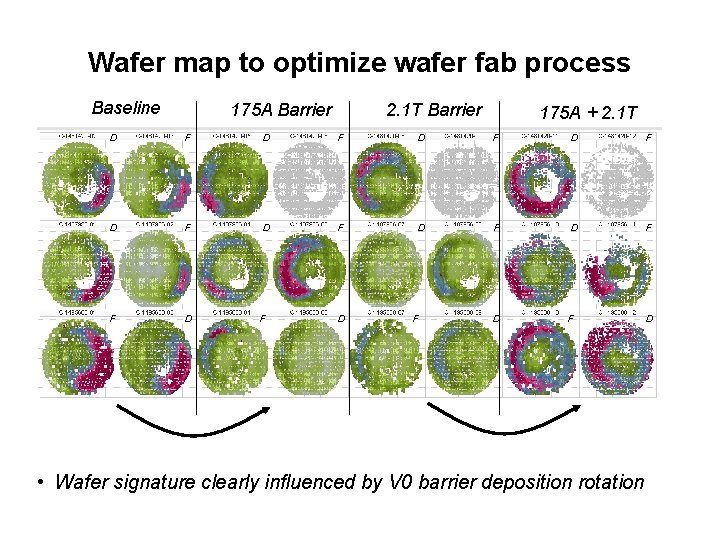
Data Visualization Tools – Wafer Maps • A wafer fail map displays the location of failing die on each probed wafer in a production lot. • A parametric wafer map displays the test result of the dies in a color or 3 dimensional manner • A wafer map helps to identify the root cause for yield loss. Fail pattern can occur by – Reticle size – multisite probe head contact (test site dependent) – Process related (with e. g. donut, ring, upper/lower half or left/right half, star or random fails) • With die Identifier on every single die, a wafer map can be re-generated based on final test data 9

• Data Visualization Tools – Wafer Maps Bin 1: Pass Bin 2: Power Supply Failures Bin 3: Digital Pattern Failures Bin 4: RECV Channel Failures Bin 5: XMIT Channel Failures Bin 7: Continuity Failures 10

RF- Wafer Probe of WLAN Frontend SIP Die Noise Figure parametric wafer map Membrane Production RF -Probe set-up

Parametric wafer map with ring performance pattern

Wafer map to optimize wafer fab process Baseline 175 A Barrier 2. 1 T Barrier 175 A + 2. 1 T D F D F F D D F • Wafer signature clearly influenced by V 0 barrier deposition rotation

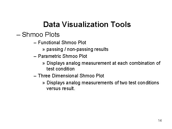
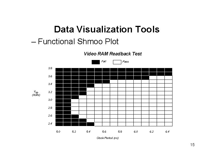
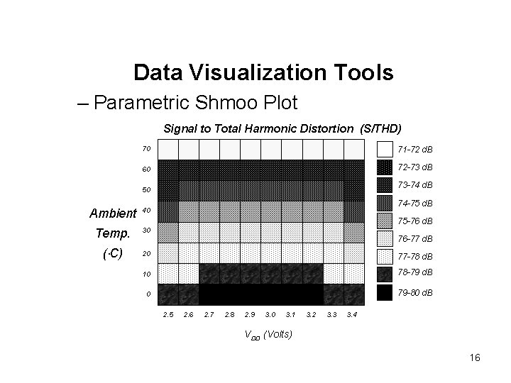
Data Visualization Tools – Shmoo Plots – Functional Shmoo Plot » passing / non-passing results – Parametric Shmoo Plot » Displays analog measurement at each combination of test condition – Three Dimensional Shmoo Plot » Displays analog measurements of two test conditions versus result. 14

Data Visualization Tools – Functional Shmoo Plot Video RAM Readback Test Fail Pass 3. 8 3. 6 3. 4 VDD (Volts) 3. 2 3. 0 2. 8 2. 6 2. 4 5. 0 5. 2 5. 4 5. 6 5. 8 6. 0 6. 2 6. 4 Clock Period (ns) 15

Data Visualization Tools – Parametric Shmoo Plot Signal to Total Harmonic Distortion (S/THD) 70 71 -72 d. B 60 72 -73 d. B 50 73 -74 d. B 74 -75 d. B Ambient 40 Temp. 30 ( C) 20 77 -78 d. B 10 78 -79 d. B 0 79 -80 d. B 75 -76 d. B 76 -77 d. B 2. 5 2. 6 2. 7 2. 8 2. 9 3. 0 3. 1 3. 2 3. 3 3. 4 VDD (Volts) 16

Statistical Analysis 17

Statistical Analysis – Mean (Average) and Standard Deviation (Variance) • One of the most useful items listed in a histogram is the population statistics. In statistics, the term “population” refers to a set of measured or calculated values of x(n). The mean m and standard deviation s are the most important of the population statistics. The mean represents the most probable value of a measured variable. • In many texts, the terms x (x-bar) and s are used to denote mean and standard deviation calculated from a finite population of values, while m and s are used to denote theoretical limits of the mean and standard deviation as the population size extends to infinity. For small populations, the values of x and s only approximate m and s. • The standard Deviation s is most useful when the population is Gaussian distributed 18

Statistical Analysis – Mean (Average) and Standard Deviation (Variance) • The standard deviation s, on the other hand, is a measure of the dispersion or uncertainty of the measured quantity about the mean value, m. • If the values tend to be concentrated near the mean, the standard deviation is small. • If the values tend to be distributed far from the mean, the standard deviation is large. • Mean and standard deviation should be evaluated together with minimum and maximum measured value • A good conclusion for non-Gaussian distributions can only be made by analyzing the entire Histogram 19

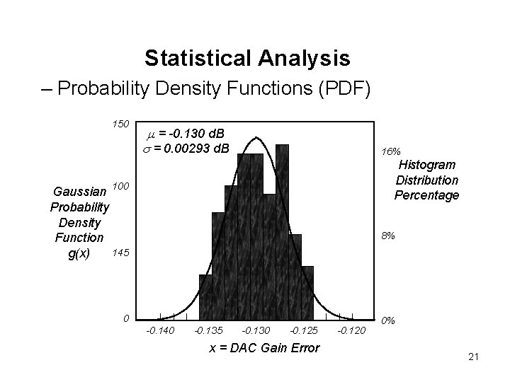
Statistical Analysis – Probability Density Functions (PDF or pdf) • According to the central limit theorem, the distribution of a set of random variables each of which is equal to a summation of a large number (N > 30) of statistically independent random values trends toward a Gaussian distribution. • As N becomes very large, the distribution of the random variables becomes Gaussian, whether or not the individual random values themselves exhibit a Gaussian distribution. • The variations in a typical mixed-signal measurement are caused by a summation of many different random sources of noise and crosstalk in both the device and the tester instruments. • As a result, many mixed-signal measurements exhibit the common Gaussian or close to Gaussian distribution 20

Statistical Analysis – Probability Density Functions (PDF) 150 m = -0. 130 d. B s = 0. 00293 d. B 16% Histogram Distribution Percentage 100 Gaussian Probability Density Function 145 g(x) 8% 0 -0. 140 -0. 135 -0. 130 -0. 125 x = DAC Gain Error -0. 120 0% 21

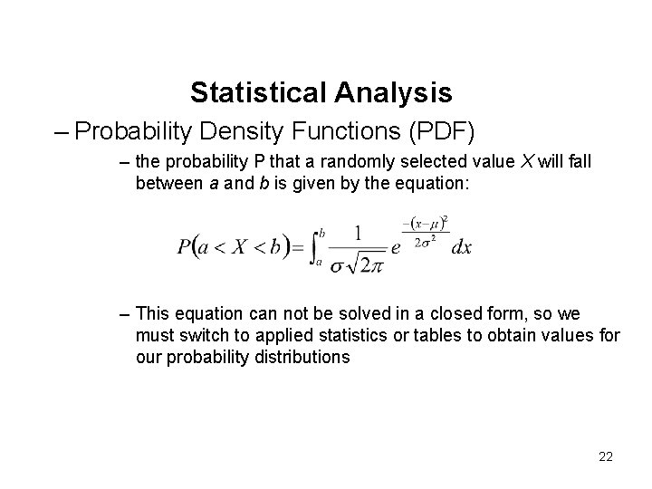
Statistical Analysis – Probability Density Functions (PDF) – the probability P that a randomly selected value X will fall between a and b is given by the equation: – This equation can not be solved in a closed form, so we must switch to applied statistics or tables to obtain values for our probability distributions 22

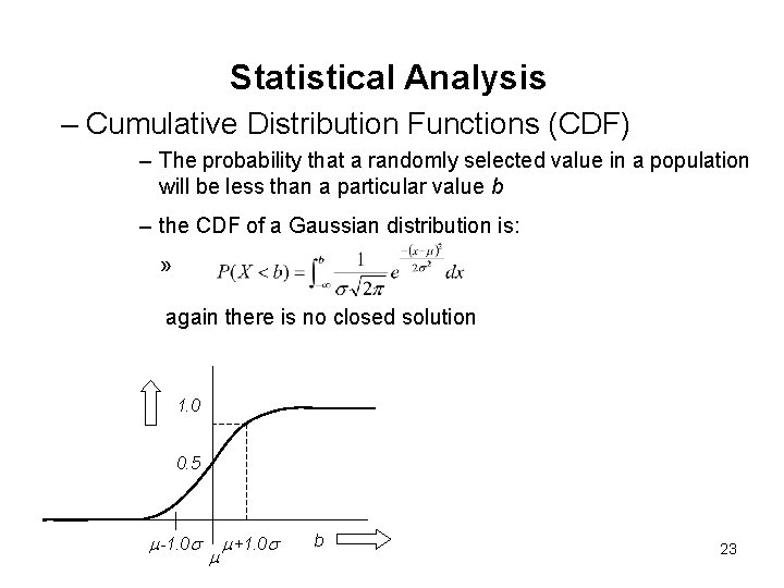
Statistical Analysis – Cumulative Distribution Functions (CDF) – The probability that a randomly selected value in a population will be less than a particular value b – the CDF of a Gaussian distribution is: » again there is no closed solution 1. 0 0. 5 m-1. 0 s m m+1. 0 s b 23

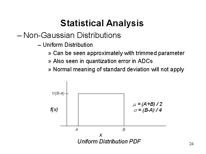
Statistical Analysis – Non-Gaussian Distributions – Uniform Distribution » Can be seen approximately with trimmed parameter » Also seen in quantization error in ADCs » Normal meaning of standard deviation will not apply 1/(B-A) m = (A+B) / 2 s = (B-A) / 4 f(x) A B x Uniform Distribution PDF 24

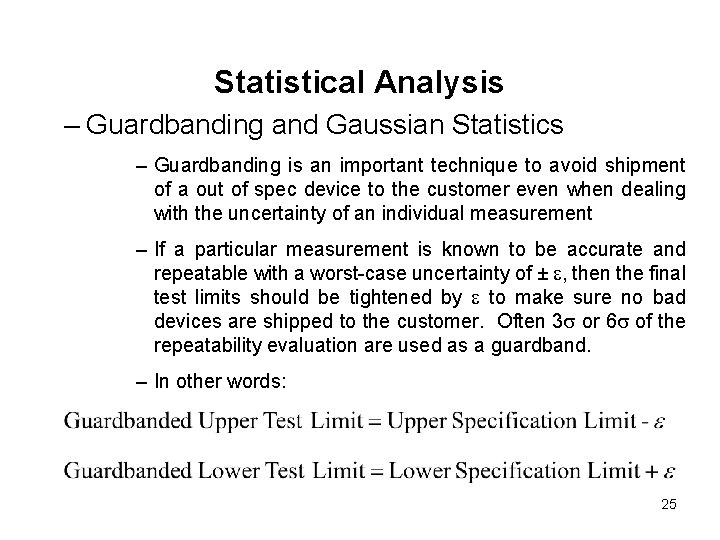
Statistical Analysis – Guardbanding and Gaussian Statistics – Guardbanding is an important technique to avoid shipment of a out of spec device to the customer even when dealing with the uncertainty of an individual measurement – If a particular measurement is known to be accurate and repeatable with a worst-case uncertainty of ± e, then the final test limits should be tightened by e to make sure no bad devices are shipped to the customer. Often 3 s or 6 s of the repeatability evaluation are used as a guardband. – In other words: 25

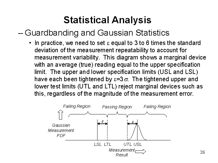
Statistical Analysis – Guardbanding and Gaussian Statistics • In practice, we need to set e equal to 3 to 6 times the standard deviation of the measurement repeatability to account for measurement variability. This diagram shows a marginal device with an average (true) reading equal to the upper specification limit. The upper and lower specification limits (USL and LSL) have each been tightened by e=3 s. The tightened upper and lower test limits (UTL and LTL) reject marginal devices such as this, regardless of the magnitude of the measurement error. Failing Region Gaussian Measurement PDF Passing Region e Failing Region e LSL LTL USL Measurement Result 26

Statistical Analysis – Guardbanding and Gaussian Statistics • If a device is well-designed and a particular measurement is sufficiently repeatable, then there will be few failures resulting from that measurement. But if the distribution of measurements from a production lot is skewed so that the average measurement is close to one of the test limits, then production yields are likely to fall. In other words, more good devices will fall within the guardband region and be disqualified. • The only way the test engineer can minimize the required guardbands is to improve the repeatability and accuracy of the test, but this requires longer test times. At some point, the test time cost of a more repeatable measurement outweighs the cost of throwing away a few good devices. 27

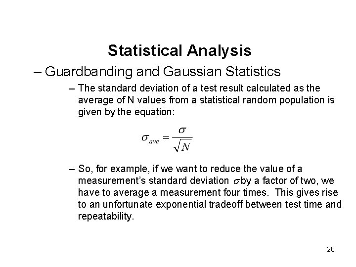
Statistical Analysis – Guardbanding and Gaussian Statistics – The standard deviation of a test result calculated as the average of N values from a statistical random population is given by the equation: – So, for example, if we want to reduce the value of a measurement’s standard deviation s by a factor of two, we have to average a measurement four times. This gives rise to an unfortunate exponential tradeoff between test time and repeatability. 28

HW How many times would we have to average a DC measurement with 27 m. V standard deviation, to achieve 6 s guardband of 10 m. V? If each measurement takes 5 ms, what would be the total test time for the averaged measurement? 29

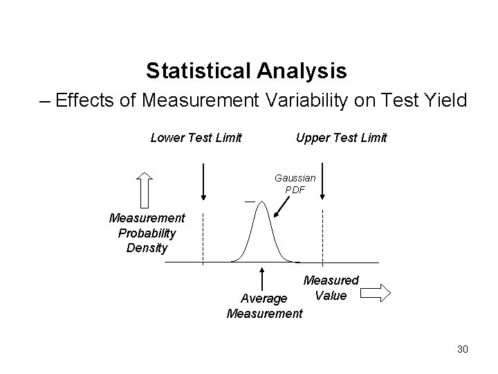
Statistical Analysis – Effects of Measurement Variability on Test Yield Lower Test Limit Upper Test Limit Gaussian PDF Measurement Probability Density Average Measurement Measured Value 30

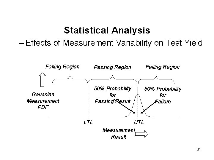
Statistical Analysis – Effects of Measurement Variability on Test Yield Failing Region Gaussian Measurement PDF LTL Passing Region Failing Region 50% Probability for Passing Result 50% Probability for Failure UTL Measurement Result 31

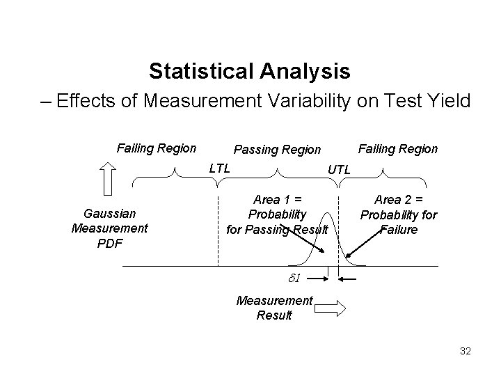
Statistical Analysis – Effects of Measurement Variability on Test Yield Failing Region LTL Gaussian Measurement PDF Failing Region Passing Region UTL Area 1 = Probability for Passing Result Area 2 = Probability for Failure d 1 Measurement Result 32

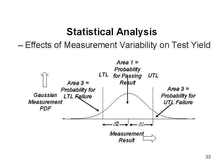
Statistical Analysis – Effects of Measurement Variability on Test Yield Area 3 = Probability for Gaussian LTL Failure Measurement PDF Area 1 = Probability LTL for Passing Result UTL Area 3 = Probability for UTL Failure d 2 d 1 Measurement Result 33

Statistical Analysis – Effects of Reproducibility and Process Variation on Yield – Factors affecting DUT parameter variation include measurement repeatability, measurement reproducibilty, and the stability of the process used to manufacture the DUT. – So far we have examined only the effects of measurement repeatability on yield, but the equations describing yield loss due to measurement variability are equally applicable to the total variability of DUT parameters. – Inaccuracies due to poor tester-to-tester correlation, day-today correlation, or DIB-to-DIB correlation appear as reproducibility errors. 34

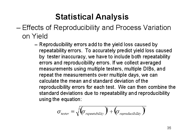
Statistical Analysis – Effects of Reproducibility and Process Variation on Yield – Reproducibility errors add to the yield loss caused by repeatability errors. To accurately predict yield loss caused by tester inaccuracy, we have to include both repeatability errors and reproducibility errors. If we collect averaged measurements using multiple testers, multiple DIBs, and repeat the measurements over multiple days, we can calculate the mean and standard deviation of the reproducibility errors for each test. We can then combine the standard deviations due to repeatability and reproducibility using the equation: 35

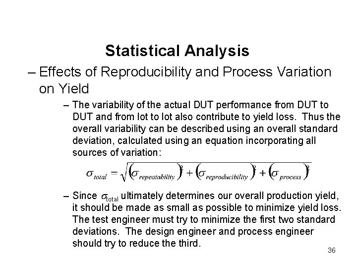
Statistical Analysis – Effects of Reproducibility and Process Variation on Yield – The variability of the actual DUT performance from DUT to DUT and from lot to lot also contribute to yield loss. Thus the overall variability can be described using an overall standard deviation, calculated using an equation incorporating all sources of variation: – Since stotal ultimately determines our overall production yield, it should be made as small as possible to minimize yield loss. The test engineer must try to minimize the first two standard deviations. The design engineer and process engineer should try to reduce third. 36

HW A six-month yield study finds that the total standard deviation of a particular DC offset measurement is 37 m. V across multiple lots, multiple testers, multiple DIB boards, etc. The standard deviation of the measurement repeatability is found to be 15 m. V, while the standard deviation of the reproducibility is found to be 7 m. V. What is the standard deviation of the actual DUT-to-DUT offset variability, excluding tester repeatability errors and reproducibility errors? If we could test this device using perfectly accurate, repeatable test equipment, what would be the total yield loss due to this parameter, assuming an average value of 2. 430 Volts and test limits of 2. 5 V 100 m. V. 37

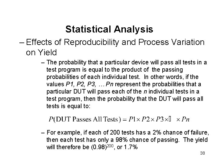
Statistical Analysis – Effects of Reproducibility and Process Variation on Yield – The probability that a particular device will pass all tests in a test program is equal to the product of the passing probabilities of each individual test. In other words, if the values P 1, P 2, P 3, … Pn represent the probabilities that a particular DUT will pass each of the n individual tests in a test program, then the probability that the DUT will pass all tests is equal to: – For example, if each of 200 tests has a 2% chance of failure, then each test has only a 98% chance of passing. The yield will therefore be (0. 98)200, or 1. 7% 38

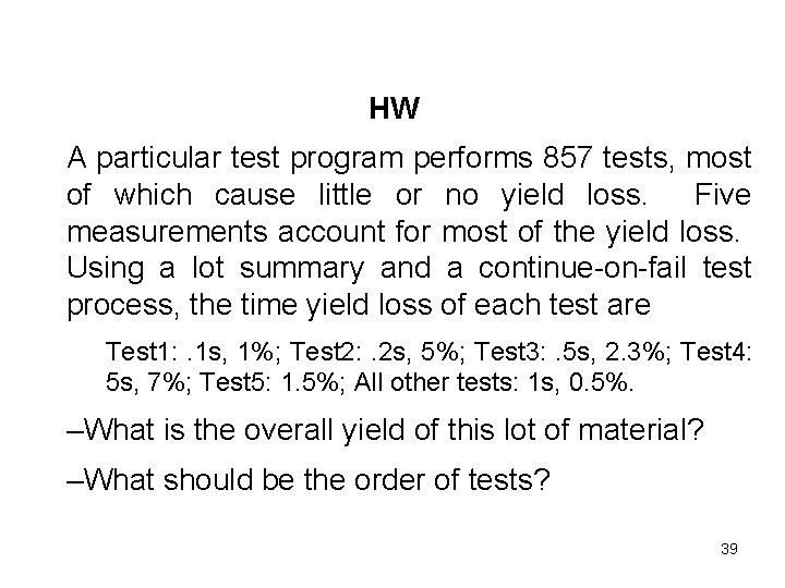
HW A particular test program performs 857 tests, most of which cause little or no yield loss. Five measurements account for most of the yield loss. Using a lot summary and a continue-on-fail test process, the time yield loss of each test are Test 1: . 1 s, 1%; Test 2: . 2 s, 5%; Test 3: . 5 s, 2. 3%; Test 4: 5 s, 7%; Test 5: 1. 5%; All other tests: 1 s, 0. 5%. –What is the overall yield of this lot of material? –What should be the order of tests? 39

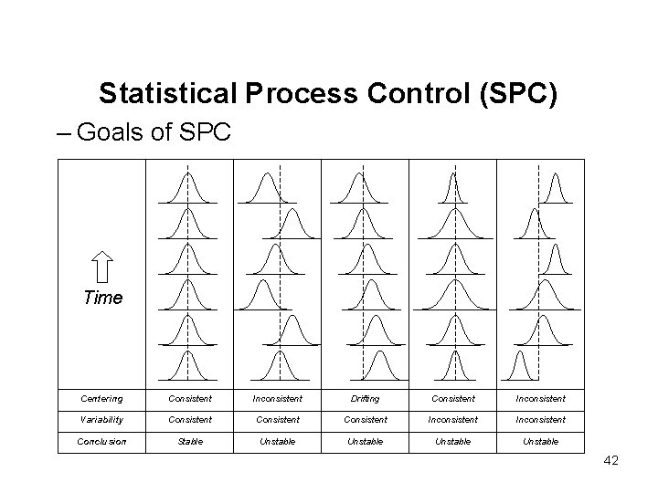
Statistical Process Control (SPC) – Goals of SPC – SPC provides a means of identifying device parameters that exhibit excessive variations over time. It does not identify the root cause of the variations, but it tells us when to look for problems. Once an unstable parameter has been identified using SPC, the engineering and manufacturing team searches for the root cause of the instability. Hopefully, the excessive variations can be reduced or eliminated through a design modification or through an improvement in one of the many manufacturing steps. By improving the stability of each tested parameter, the manufacturing process is brought under control, enhancing the inherent quality of the product. 40

Statistical Process Control (SPC) – Goals of SPC – Once the stability of the distributions has been verified, the parameter might only be measured for every tenth device or every hundredth device in production. If the mean and standard deviation of the limited sample set stays within tolerable limits, then we can be confident that the manufacturing process itself is stable. SPC thus allows statistical sampling of highly stable parameters, dramatically reducing testing costs. 41

Statistical Process Control (SPC) – Goals of SPC Time Centering Consistent Inconsistent Drifting Consistent Inconsistent Variability Consistent Inconsistent Conclusion Stable Unstable 42

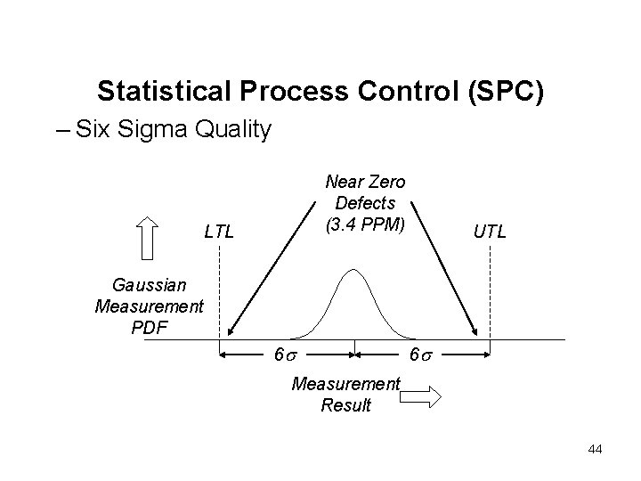
Statistical Process Control (SPC) – Six Sigma Quality – If successful, the SPC process results in an extremely small percentage of parametric test failures. The ultimate goal of SPC is to achieve six-sigma quality standards for each specified device parameter. – A parameter is said to meet six-sigma quality standards if the center of its statistical distribution is at least 6 s away from the upper and lower test limits. – Six-sigma quality standards result in a failure rate of only 3. 4 parts per million (ppm). Therefore, the chance of an untested device failing a six-sigma parameter is extremely low. – This is the reason we can often eliminate DUT-by-DUT testing of six-sigma parameters. 43

Statistical Process Control (SPC) – Six Sigma Quality Near Zero Defects (3. 4 PPM) LTL UTL Gaussian Measurement PDF 6 s 6 s Measurement Result 44

Statistical Process Control (SPC) – Process Capability, Cp and Cpk – Process capability is the inherent variation of the process used to manufacture a product. Process capability is defined as the 3 s variation of a parameter around its mean value. For example, if a given parameter exhibits a 10 m. V standard deviation from DUT to DUT over a period of time, then the process capability for this parameter is defined as 60 m. V. 45

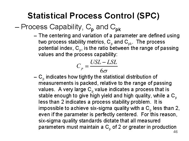
Statistical Process Control (SPC) – Process Capability, Cp and Cpk – The centering and variation of a parameter are defined using two process stability metrics, Cp and Cpk. The process potential index, Cp, is the ratio between the range of passing values and the process capability: – Cp indicates how tightly the statistical distribution of measurements is packed, relative to the range of passing values. A very large Cp value indicates a process that is stable enough to give high yield and high quality, while a Cp less than 2 indicates a process stability problem. It is impossible to achieve six-sigma quality with a Cp less than 2, even if the parameter is perfectly centered. For this reason, six-sigma quality standards dictate that all measured parameters must maintain a Cp of 2 or greater in production 46

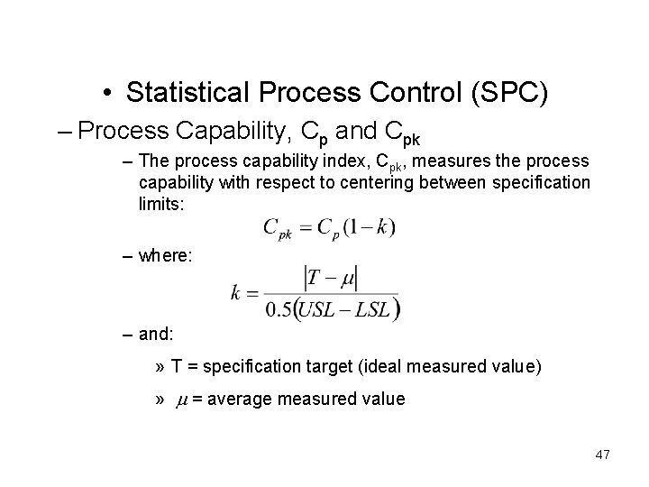
• Statistical Process Control (SPC) – Process Capability, Cp and Cpk – The process capability index, Cpk, measures the process capability with respect to centering between specification limits: – where: – and: » T = specification target (ideal measured value) » m = average measured value 47

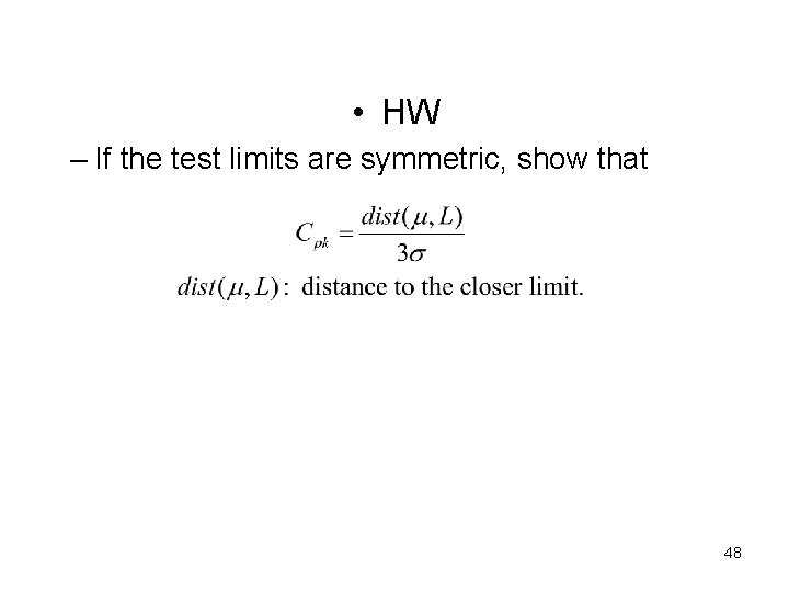
• HW – If the test limits are symmetric, show that 48

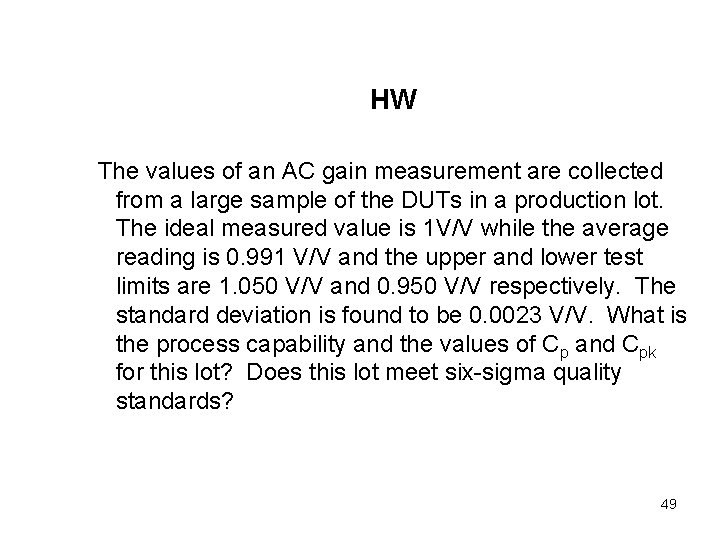
HW The values of an AC gain measurement are collected from a large sample of the DUTs in a production lot. The ideal measured value is 1 V/V while the average reading is 0. 991 V/V and the upper and lower test limits are 1. 050 V/V and 0. 950 V/V respectively. The standard deviation is found to be 0. 0023 V/V. What is the process capability and the values of Cp and Cpk for this lot? Does this lot meet six-sigma quality standards? 49

Statistical Process Control (SPC) – Gauge Repeatability and Reproducibility – As mentioned previously in this chapter, a measured parameter’s variation is partially due to variations in the materials and the process used to fabricate the device and partially due to the tester’s repeatability errors and reproducibility errors. In the language of SPC, the tester is known as a gauge. Before we can apply SPC to a manufacturing process, we first need to verify the accuracy, repeatability, and reproducibility of the gauge. Once the quality of the testing process has been established, the test data collected during production can be continuously monitored to verify a stable manufacturing process. 50

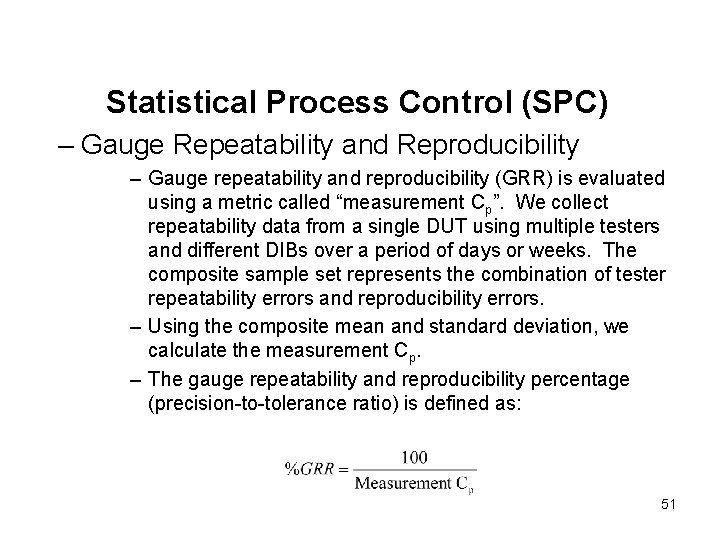
Statistical Process Control (SPC) – Gauge Repeatability and Reproducibility – Gauge repeatability and reproducibility (GRR) is evaluated using a metric called “measurement Cp”. We collect repeatability data from a single DUT using multiple testers and different DIBs over a period of days or weeks. The composite sample set represents the combination of tester repeatability errors and reproducibility errors. – Using the composite mean and standard deviation, we calculate the measurement Cp. – The gauge repeatability and reproducibility percentage (precision-to-tolerance ratio) is defined as: 51

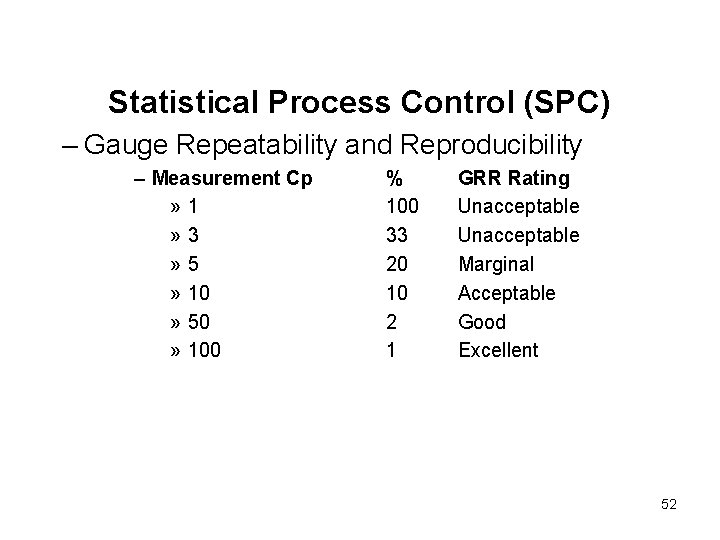
Statistical Process Control (SPC) – Gauge Repeatability and Reproducibility – Measurement Cp » 1 » 3 » 5 » 10 » 50 » 100 % 100 33 20 10 2 1 GRR Rating Unacceptable Marginal Acceptable Good Excellent 52

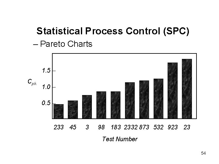
Statistical Process Control (SPC) – Pareto Charts – A Pareto chart is a graph of values in ascending or descending order of importance. Pareto charts help us identify the most significant factors in a sea of data. For example, we may wish to concentrate our process improvement efforts on the ten parameters that have the lowest Cpk values. We can plot the value of Cpk for every parameter in a test program, starting with the lowest and progressing toward the highest. If we have hundreds of tests, this technique allows us to quickly isolate the tests having the worst centering and variability. 53

Statistical Process Control (SPC) – Pareto Charts 1. 5 Cpk 1. 0 0. 5 233 45 3 98 183 2332 873 532 923 23 Test Number 54

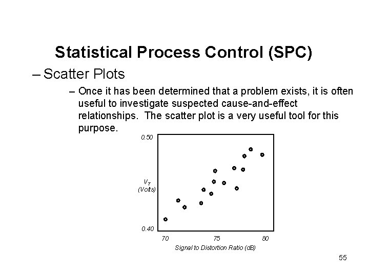
Statistical Process Control (SPC) – Scatter Plots – Once it has been determined that a problem exists, it is often useful to investigate suspected cause-and-effect relationships. The scatter plot is a very useful tool for this purpose. 0. 50 VT (Volts) 0. 40 70 75 80 Signal to Distortion Ratio (d. B) 55

Statistical Process Control (SPC) – Scatter Plots – If all the points in a scatter plot form a line, then there is a strong correlation between the factors. If they are randomly placed throughout the chart, then there is no correlation. As the example scatter plot shows, the threshold voltage and distortion exhibit a fairly strong correlation. The engineering team would then know that the distortion parameter might be stabilized by stabilizing the transistor threshold voltage. 56

Statistical Process Control (SPC) – Control Charts – In addition to monitoring the Cp and Cpk of critical parameters, we can also monitor the stability of a process using control charts. A control chart is a graph of parameter stability over time. An effective SPC implementation depends in large part on selecting the appropriate critical parameters to monitor and then choosing an appropriate set of control charts. Control charts are the mechanism by which we determine when the quality metric of interest is drifting out of control. 57

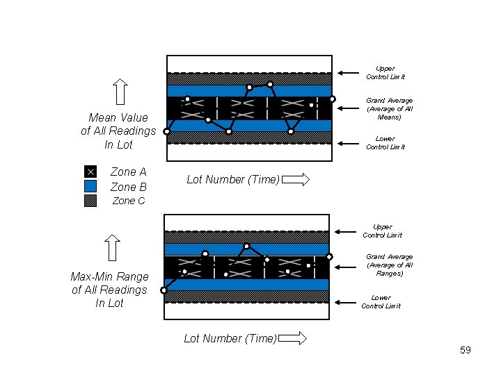
Statistical Process Control (SPC) – Control Charts – For example, we may choose to monitor the mean and range (range = maximum reading – minimum reading) of a particular parameter for each production lot. We can track the fluctuations in these mean and range values over time, creating an X-Bar control chart and a range control chart. We then define upper and lower control limits for each chart. 58

Upper Control Limit Grand Average (Average of All Means) Mean Value of All Readings In Lot Zone A Zone B Lower Control Limit Lot Number (Time) Zone C Upper Control Limit Grand Average (Average of All Ranges) Max-Min Range of All Readings In Lot Lower Control Limit Lot Number (Time) 59

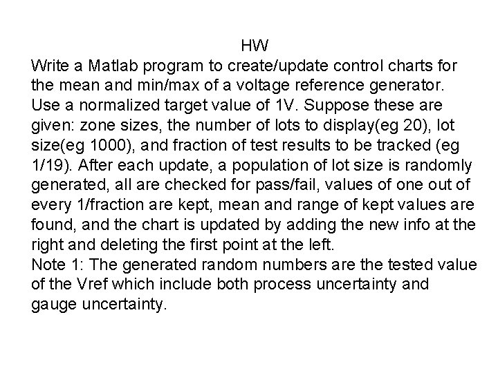
HW Write a Matlab program to create/update control charts for the mean and min/max of a voltage reference generator. Use a normalized target value of 1 V. Suppose these are given: zone sizes, the number of lots to display(eg 20), lot size(eg 1000), and fraction of test results to be tracked (eg 1/19). After each update, a population of lot size is randomly generated, all are checked for pass/fail, values of one out of every 1/fraction are kept, mean and range of kept values are found, and the chart is updated by adding the new info at the right and deleting the first point at the left. Note 1: The generated random numbers are the tested value of the Vref which include both process uncertainty and gauge uncertainty.

HW (continued) Note 2: The max/min zones, the mean zones are related to USL/LSL, how? The lot size, fraction and total uncertainty affect the mean zone sizes. The total uncertainty is determined from USL/LSL, Cp, and GRR. Derive these relations and use them to write your code. Note 3: you can make your program to be continuously running, until ctrl-c is pressed. Note 4: You can add some instability in your process and/or gauge uncertainty (m, s), but do this either slowly or piecewise constant over multiple lots.

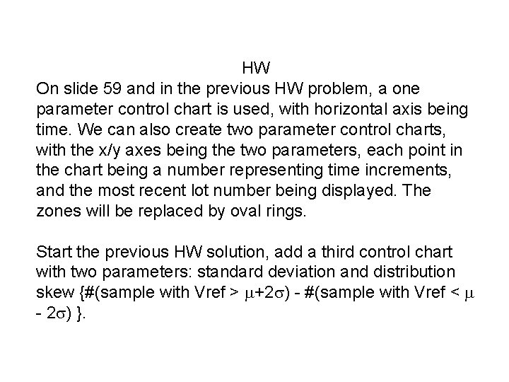
HW On slide 59 and in the previous HW problem, a one parameter control chart is used, with horizontal axis being time. We can also create two parameter control charts, with the x/y axes being the two parameters, each point in the chart being a number representing time increments, and the most recent lot number being displayed. The zones will be replaced by oval rings. Start the previous HW solution, add a third control chart with two parameters: standard deviation and distribution skew {#(sample with Vref > m+2 s) - #(sample with Vref < m - 2 s) }.

Summary • There are literally hundreds if not thousands of ways to view and process data gathered during the production testing process. In this chapter, we have examined only a few of the more common data displays, such as the datalog, wafer map, scatter plot, and histogram. Using statistical analysis, we can predict the effects of a parameter’s variation on the overall test yield of a product. We can also use statistical analysis to evaluate the repeatability and reproducibility of the measurement equipment itself. 63

Summary (cont) • Statistical process control allows us to not only evaluate the quality of the process, including the test and measurement equipment, but it tells us when the manufacturing process is not stable. We can then work to fix or improve the manufacturing process to bring it back under control. 64