Introduction to Computer Simulation of Physical Systems Lecture

Introduction to Computer Simulation of Physical Systems (Lecture 7) The Chaotic Motion of Dynamical Systems PHYS 3061

Recall the equation introduced last time • natural to formulate a more realistic model – the population is bounded by the finite carrying capacity of its environment. – A simple model of density-dependent growth is Pn+1 = Pn(a − b. Pn).

• convenient to rescale the population – by letting Pn = (a/b)xn – xn+1 = axn(1 − xn) • The replacement of Pn by xn changes the units. • In the standard form, – the parameter r = a/4 – And xn+1 = f(xn) = 4 rxn(1 − xn). • that x is restricted to the interval 0 ≤ x ≤ 1 and 0 < r ≤ 1.

• The form of f(x) is known as the logistic map. • The logistic map is a simple example of a dynamical system, – the map is a deterministic, mathematical prescription for finding the future state of a system given its present state.

• The first thirty iterations are shown for two values of r here.

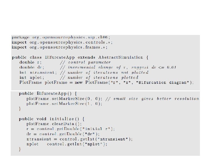
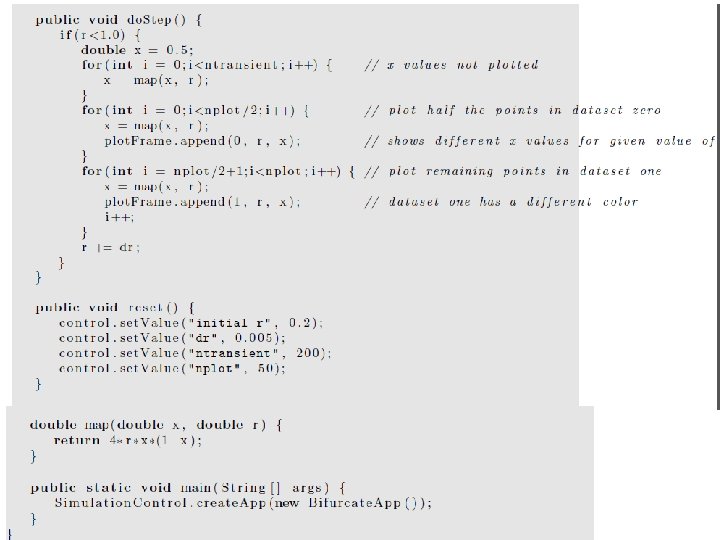
• Plot the values of x as a function of r. • The iterated values of x are plotted after the initial transient behavior is discarded.

• For each value of r, – the first n transient values of x are computed – but not plotted. – Then the next nplot values of x are plotted, • with the first half in one color and the second half in another. • This process is repeated – for a new value of r until the desired range of r values is reached. • The magnitude of nplot – at least as large as the longest period that you wish to observe. • Bifurcate. App extends Abstract. Simulation rather than Abstract. Calculation because the calculations can be time consuming, and you might want to stop them before they are finished and reset some of the parameters.

Period Doubling • The results of the numerical experiments shows that – the dynamical properties of a simple nonlinear deterministic system can be quite complicated. • To gain more insight into how the dynamical behavior depends on r, – we introduce a simple graphical method. – We show a graph of f(x) versus x for r = 0. 7. • A diagonal line corresponding to y = x intersects the curve y = f(x) at the two fixed points x∗ = 0 and x∗ = 9/14 ≈ 0. 642857.

• • • If x 0 is not a fixed point, we can find the trajectory in the following way. Draw a vertical line from (x = x 0, y = 0) to the intersection with the curve y = f(x) at (x 0, y 0 = f(x 0)). Next draw a horizontal line from (x 0, y 0) to the intersection with the diagonal line at (y 0, y 0). On this diagonal line y = x, and hence the value of x at this intersection is the first iteration x 1 = y 0. The second iteration x 2 can be found in the same way. From the point (x 1, y 0), draw a vertical line to the intersection with the curve y = f(x). Keep y fixed at y = y 1 = f(x 1), and draw a horizontal line until it intersects the diagonal line; the value of x at this intersection is x 2. Further iterations can be found by repeating this process. Any observations of fixed points on this graph?

• If we begin with any x 0 (except x 0 = 0 and x 0 = 1), the iterations will converge to the fixed point x∗ ≈ 0. 643. • It would be a good idea to repeat the procedure by hand. • For r = 0. 7, the fixed point is stable (an attractor of period 1). • In contrast, no matter how close x 0 is to the fixed point at x = 0, the iterates diverge away from it, and this fixed point is unstable.

• How can we explain the qualitative difference between the fixed point at x = 0 and at x∗ = 0. 642857 for r = 0. 7? • The local slope of the curve y = f(x) determines that the distance moved horizontally each time f is iterated. • A slope steeper than 45◦ leads to a value of x further away from its initial value. • Hence, the criterion for the stability of a fixed point is that the magnitude of the slope at the fixed point must be less than 45◦. • That is, if |df(x)/dx|x=x∗ is less than unity, then x∗ is stable; • conversely, if |df(x)/dx|x=x∗ is greater than unity, then x∗ is unstable.

• An inspection of f(x) shows that – x = 0 is unstable because the slope of f(x) at x = 0 is greater than unity. – In contrast, the magnitude of the slope of f(x) at x = x∗ ≈ 0. 643 is less than unity and this fixed point is stable. • x∗= 0 is stable for 0 < r < 1/4, and • x∗= 1 − 1/4 r is stable for 1/4 < r < 3/4.

• What happens if r is greater than 3/4? • If r is slightly greater than 3/4, the fixed point of f becomes unstable and bifurcates to a cycle of period 2. • Now x returns to the same value after every second iteration, and the fixed points of • f(f(x))are the stable attractors of f(x). • In the following, we write f(2)(x) = f(f(x)) and f(n)(x) for the nth iterate of f(x). – (Do not confuse f(n)(x) with the nth derivative of f(x). )

• For example, the second iterate f(2)(x) is given by the fourth-order polynomial:

• What happens if we increase r still further? • Eventually the magnitude of the slope of the fixed points of f(2)(x) exceeds unity and the fixed points of f(2)(x) become unstable. • Now the cycle of f is period 4, and the fixed points of the fourth iteration • f(4)(x) = f(2)(x))= f(f(x))) are stable. • These fixed points also eventually become unstable, and we are led to the phenomena of period doubling

Read the text book for the code of Graphical. Solution. App, which displays the graphical solution of the logistic map trajectory

• Periodic windows in the chaotic regime. • At the bifurcation diagram, you will see that the range of chaotic behavior for r > r∞ is interrupted by intervals of periodic behavior. • Magnify the bifurcation diagram, at the interval 0. 957107 ≤ r ≤ 0. 960375, – a periodic trajectory of period 3 occurs. – (Period 3 behavior starts at r = (1 +√ 8)/4. ) • An example of intermittency, that is, nearly periodic behavior interrupted by occasional irregular bursts.

Universal Properties and Self. Similarity • In Sections 2 and 3 we found that the trajectory of the logistic map has remarkable properties – as a function of the control parameter r. • A sequence of period doublings accumulating in a chaotic trajectory of infinite period at r = r∞. • For most values of r > r∞, the trajectory is very sensitive to the initial conditions.

• We also found “windows” of period 3, 6, 12, . . . embedded in the range of chaotic behavior. • How typical is this type of behavior? • further numerical evidence will show that the general behavior of the logistic map is independent of the details of the form of f(x).

• Noticed that the range of r between successive bifurcations becomes smaller as the period increases. – For example, b 2 − b 1 = 0. 112398, b 3 − b 2 = 0. 023624, and b 4 − b 3 = 0. 00508. – A good guess is that the decrease in bk − bk− 1 is geometric, that is, the ratio (bk − bk− 1)/(bk+1 − bk) is a constant. – You can check that this ratio is not exactly constant, but converges to a constant with increasing k.

• This behavior suggests that the sequence of values of bk has a limit and follows a geometrical progression: • bk ≈ r∞ − C δ−k, • where δ is known as the Feigenbaum number and C is a constant. • δ is given by the ratio δ = lim (bk − bk− 1)/(bk+1 − bk), when k→∞.

• Mitchell Jay Feigenbaum (born December 19, 1944) is a mathematical physicist whose pioneering studies in chaos theory led to the discovery of the Feigenbaum constants. • In 1975, Dr. Feigenbaum, using the small HP-65 calculator he had been issued, discovered that the ratio of the difference between the values at which successive period-doubling bifurcations occur tends to a constant of around 4. 6692. . .

• We can associate another number with the series of “pitchfork” bifurcations. • Each pitchfork bifurcation gives birth to “twins” with the new generation more densely packed than the previous generation. • One measure of this density is the maximum distance Mk between the values of x describing the bifurcation

• The disadvantage of using Mk is that the transient behavior of the trajectory is very long at the boundary between two different periodic behaviors. • A more convenient measure of the distance is the quantity dk =xk∗ − 1/2, – where xk* is the value of the fixed point nearest to the fixed point x∗ = 1/2. • The first two values of dk are shown in Figure here with d 1 ≈ 0. 3090 and d 2 ≈ − 0. 1164. • The next value is d 3 ≈ 0. 0460. • Note that the fixed point nearest to x = 1/2 alternates from one side of x = 1/2 to the other.

• We define the quantity α by the ratio α = limk→∞−( dk/dk+1). • The ratios α = (0. 3090/0. 1164) = 2. 65 for k = 1 • and α = (0. 1164/0. 0460) = 2. 53 for k = 2 are consistent with the asymptotic value α = 2. 5029078750958928485. . .

• qualitative arguments: – that suggest that the general behavior of the logistic map in the period doubling regime is independent of the detailed form of f(x). • doubling is characterized by self-similarities, – for example, the period doublings look similar except for a change of scale. – We can demonstrate these similarities by comparing f(x) for r = s 1 = 0. 5 for the superstable trajectory with period 1 to the function f(2) (x) for r = s 1 ≈ 0. 809017 for the superstable trajectory of period 2

• The function f(x, r = s 1) has unstable fixed points at x = 0 and x = 1 and a stable fixed point at x = 1/2. • Similarly the function f(2)(x, r = s 2) has a stable fixed point at x = 1/2 and an unstable fixed point at x ≈ 0. 69098. • Note the similar shape, but different scale of the curves in the square boxes.

• This similarity is an example of scaling. • That is, if we scale f(2) and change (renormalize) the value of r, we can compare f(2) to f. • This graphical comparison is only suggestive.

• A precise approach shows that if we continue the comparison of the higher-order iterates, for example, f(4)(x) to f(2)(x), etc. , the superposition of functions converges to a universal function that is independent of the form of the original function f(x).

• Why is the universality of period doubling and the numbers δ and α more than a curiosity? • The reason is that because this behavior is independent of the details, there might exist realistic systems whose underlying dynamics yield the same behavior as the logistic map. • Of course, most physical systems are described by differential rather than difference equations.

• Can these systems exhibit period doubling behavior? • Several workers (cf. Testa et al. ) have constructed nonlinear RLC circuits driven by an oscillatory source voltage. • The output voltage shows bifurcations, and the measured values of the exponents δ and α are consistent with the predictions of the logistic map.

• the nature of turbulence in fluid systems. • Consider a stream of water flowing past several obstacles. • At low flow speeds, the water flows past obstacles in a regular and time-independent fashion, called laminar flow. • As the flow speed is increased (as measured by a dimensionless parameter called the Reynolds number), some swirls develop, but the motion is still time-independent. • As the flow speed is increased still further, the swirls break away and start moving downstream. • The flow pattern as viewed from the bank becomes timedependent. • For still larger flow speeds, the flow pattern becomes very complex and looks random. We say that the flow pattern has made a transition from laminar flow to turbulent flow.

• This qualitative description of the transition to chaos in fluid systems is superficially similar to the description of the logistic map. • Can fluid systems be analyzed in terms of the simple models of the type we have discussed here? • In a few instances such as turbulent convection in a heated saucepan, period doubling and other types of transitions to turbulence have been observed. • The type of theory and analysis we have discussed has suggested new concepts and approaches, and the study of turbulent flow is a subject of much current interest.

Measuring Chaos • How do we know if a system is chaotic? • The most important characteristic of chaos is sensitivity to initial conditions. • We found that the trajectories starting from x 0 = 0. 5 and x 0 = 0. 5001 for r = 0. 91 become very different after a small number of iterations.

• Computers only store floating numbers to a certain number of digits, – the implication of this result: our numerical predictions of the trajectories of chaotic systems are restricted to small time intervals. • Sensitivity to initial conditions implies that even though the logistic map is deterministic, our ability to make numerical predictions of its trajectory is limited.

• How can we quantify this lack of predictably? • In general, if we start two identical dynamical systems from slightly different initial conditions, we expect that the difference between the trajectories will increase as a function of n.

• In Figure here we show a plot of the difference |Δxn| versus n. • We see that roughly speaking, ln |Δxn| is a linearly increasing function of n. • This result indicates that the separation between the trajectories grows exponentially if the system is chaotic.

• This divergence of the trajectories can be described by the Lyapunov exponent λ, which is defined by the relation: • |Δxn| = |Δx 0| eλn, where Δxn is the difference between the trajectories at time n. • If the Lyapunov exponent λ is positive, then nearby trajectories diverge exponentially. • Chaotic behavior is characterized by the exponential divergence of nearby trajectories. • Any suggestions on how to measure it?

• A naive way of measuring the Lyapunov exponent λ is to run the same dynamical system twice with slightly different initial conditions and measure the difference of the trajectories as a function of n. • Because the rate of separation of the trajectories might depend on the choice of x 0, a better method would be to compute the rate of separation for many values of x 0. • This method would be tedious, because we would have to fit the separation for each value of x 0 and then determine an average value of λ.

• A more important limitation of the naive method is that because the trajectory is restricted to the unit interval, – the separation |Δxn| ceases to increase when n becomes sufficiently large. • Fortunately, there is a better way of determining λ.

• We take the natural logarithm of both sides of the definition and write λ as • λ =1/n ln |Δxn/Δx 0|. • Because we want to use the data from the entire trajectory after the transient behavior has ended, we use the fact that

• The form above implies that we can interpret xi for any i as the initial condition. • The problem of computing λ has been reduced to finding the ratio Δxi+1/Δxi. • Because we want to make the initial difference between the two trajectories as small as possible, we are interested in the limit Δxi → 0.

• The idea of the more sophisticated procedure is to compute dxi+1/dxi from the equation of motion at the same time that the equation of motion is being iterated. • We use the logistic map as an example. • We have dxi+1/dxi= f′(xi) = 4 r(1 − 2 xi).

• We can consider xi for any i as the initial condition and the ratio dxi+1/dxi as a measure of the rate of change of xi. • Hence, we can iterate the logistic map as before and use the values of xi and the relation to compute f′(xi) = dxi+1/dxi at each iteration. • The Lyapunov exponent is given by

• we begin the sum in the above equation after the transient behavior is finished. • We have included explicitly the limit n → ∞ to remind ourselves to choose n sufficiently large. • Note that this procedure weights the points on the attractor correctly, that is, if a particular region of the attractor is not visited often by the trajectory, it does not contribute much to the sum.

• We have found that nearby trajectories diverge if λ > 0. • For λ < 0, the two trajectories converge and the system is not chaotic. • What happens for λ = 0? In this case we will see that the trajectories diverge algebraically, that is, as a power of n. • In some cases a dynamical system is at the “edge of chaos” where the Lyapunov exponent vanishes. • Such systems are said to exhibit weak chaos to distinguish their behavior from the strongly chaotic behavior (λ > 0) that we have been discussing.

• If we define z ≡ |Δxn|/|Δx 0|, then z will satisfy the differential equation dz/dn = λqzq. • For weak chaos we do not find an exponential divergence, – but instead a divergence that is algebraic and is given by – dz/dn= λqzq, – where q is a parameter that needs to be determined. • The solution is z = [1 + (1 − q)λqn]1/(1 -q), • In the limit q → 1, we recover the usual exponential dependence.

• We can determine the type of chaos using the crude approach of choosing a large number of initial values of x 0 and x 0 + Δx 0 and plotting the average of ln z versus n. • If we do not obtain a straight line, then the system does not exhibit strong chaos. • How can we check for the behavior shown in the above equation? The easiest way is to plot the quantity (Z 1 -q -1 )/ (1 -q) versus n.

• A system of fixed energy (and number of particles and volume) has an equal probability of being in any microstate specified by the positions and velocities of the particles. • One way of measuring the ability of a system to be in any state is to measure its entropy defined by S = −Σpi ln pi, – where the sum is over all states and pi is the probability or relative frequency of being in the ith state. • For example, if the system is always in only one state, then S = 0, the smallest possible entropy. • If the system explores all states equally, then S = ln Ω, where Ω is the number of possible states.

• to compute S for the logistic map, we can divide the interval [0, 1] into bins or • subintervals of width Δx = 0. 01 and determine the relative number of times the trajectory falls into each bin. • At each value of r in the range 0. 7 ≤ r ≤ 1, the map should be iterated for a fixed number of steps, for example, n = 1000. Choose Δx = 0. 01.

• We also can measure the (generalized) entropy as a function of time. • S(n) for strong chaos increases linearly with n until all the possible states are visited. • However, for weak chaos this behavior is not found. • In the latter case we can generalize the entropy to a q-dependent function defined by