Introduction to Computer Science Unit 14 l Searching

Introduction to Computer Science Unit 14 l Searching l Sorting l Complexity and Performance

Sorting and Searching l We’ve learned about arrays (one dimensional and two dimensional) l We’ve learned how to move through arrays, filling them up or printing them out l Two of the most common operations on arrays are u. Sorting: placing elements in a given order u. Searching: finding where, or if, an element appears in an array 14 - 2

Sorting and Searching l This is a widely studied problem l We’ll look at several different algorithms for carrying out sorting and searching l Five different search methods, for sorted and unsorted arrays of values l Three l And different sorting methods later, a recursive sorting method! 14 - 3

The Framework final int MAX = 10; int[ ] counts = new int[MAX]; void Initialize (int[ ] data) {…} //Loads data with test information int Search. Method (int[ ] data, // what we search int num) // what we seek {…} //Returns position of num in data, or -1 if absent void Sort. Method (int[ ] data) {…} //Sorts the array, if necessary. 14 - 4

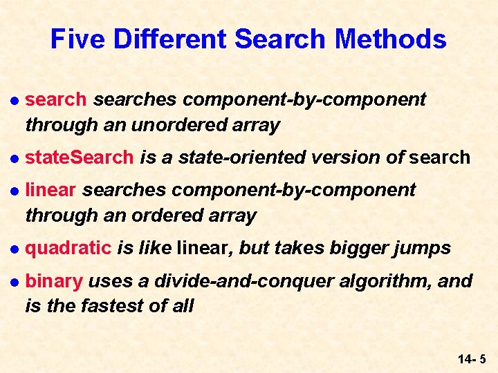
Five Different Search Methods l searches component-by-component through an unordered array l state. Search is a state-oriented version of search l linear searches component-by-component through an ordered array l quadratic is like linear, but takes bigger jumps l binary uses a divide-and-conquer algorithm, and is the fastest of all 14 - 5

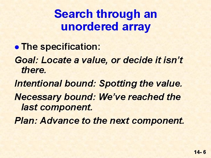
Search through an unordered array l The specification: Goal: Locate a value, or decide it isn’t there. Intentional bound: Spotting the value. Necessary bound: We’ve reached the last component. Plan: Advance to the next component. 14 - 6

The search Java Code int search (int[ ] data, int num) { // Search method for an unordered array. // Return -1 for absent number. int pos = 0; // position of current component while ( (data[pos] != num) && (pos <(data. length - 1)) ) pos++; //Postcondition: if data[pos] isn’t num, no component is. if (data[pos] == num) return pos; else return -1; } // end of search note the ambiguous postcondition 14 - 7

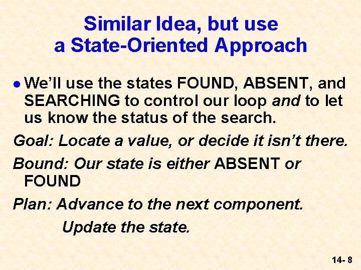
Similar Idea, but use a State-Oriented Approach l We’ll use the states FOUND, ABSENT, and SEARCHING to control our loop and to let us know the status of the search. Goal: Locate a value, or decide it isn’t there. Bound: Our state is either ABSENT or FOUND Plan: Advance to the next component. Update the state. 14 - 8

The state. Search Java Code int state. Search(int[ ] data, int num) { // State-oriented search of unordered array. Return -1 for absent num final int FOUND = 0, ABSENT = 1, SEARCHING = 2; int pos = 0, state = SEARCHING; do { // until we’re not searching anymore if (pos >= data. length) state = ABSENT; else if (data[pos] == num) state = FOUND; else pos++; } while ( state == SEARCHING) ; //Postcondition: if num was there, state’s FOUND and data[pos] is num switch (state) { case FOUND: return pos; case ABSENT: return -1; } } // end of state. Search 14 - 9

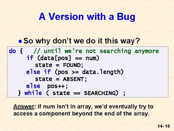
A Version with a Bug l So why don’t we do it this way? do { // until we’re not searching anymore if (data[pos] == num) state = FOUND; else if (pos >= data. length) state = ABSENT; else pos++; } while ( state == SEARCHING) ; Answer: if num isn’t in array, we’d eventually try to access a component beyond the end of the array. 14 - 10

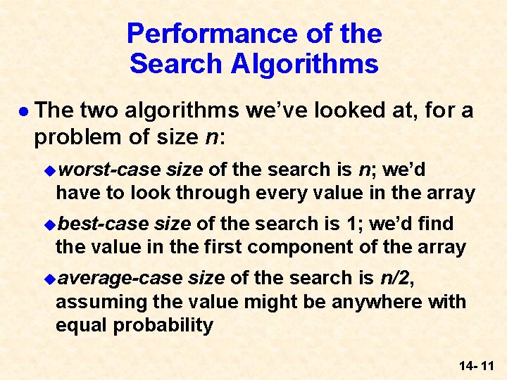
Performance of the Search Algorithms l The two algorithms we’ve looked at, for a problem of size n: uworst-case size of the search is n; we’d have to look through every value in the array ubest-case size of the search is 1; we’d find the value in the first component of the array uaverage-case size of the search is n/2, assuming the value might be anywhere with equal probability 14 - 11

Searching Ordered Arrays l When we had unordered arrays, we had to look through (potentially) every component to find the value we were looking for l With ordered arrays, we can be more clever; we look at three techniques: ulinear uquadratic ubinary 14 - 12

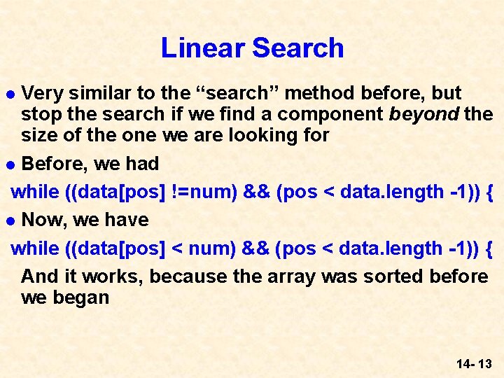
Linear Search Very similar to the “search” method before, but stop the search if we find a component beyond the size of the one we are looking for l Before, we had while ((data[pos] !=num) && (pos < data. length -1)) { l Now, we have while ((data[pos] < num) && (pos < data. length -1)) { And it works, because the array was sorted before we began l 14 - 13

The linear Java Code int linear (int[ ] data, int num) { // Linear search for num in an ordered array. // Return -1 for absent letter. int pos = 0; // position of current component while ( (data[pos]< num) && (pos < (data. length - 1)) ) pos++; //Postcondition: if data[pos] isn’t num, no component is. if (data[pos] == num) return pos; else return -1; } // end of linear 14 - 14

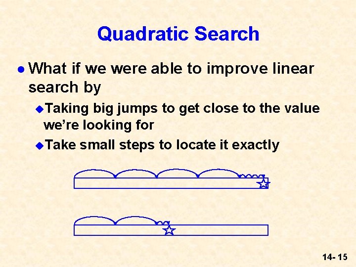
Quadratic Search l What if we were able to improve linear search by u. Taking big jumps to get close to the value we’re looking for u. Take small steps to locate it exactly 14 - 15

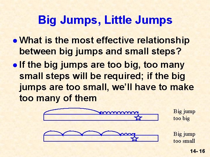
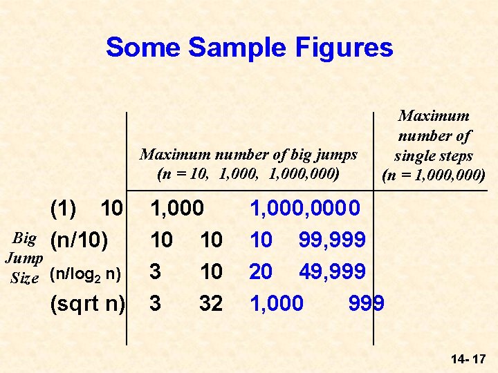
Big Jumps, Little Jumps l What is the most effective relationship between big jumps and small steps? l If the big jumps are too big, too many small steps will be required; if the big jumps are too small, we’ll have to make too many of them Big jump too big Big jump too small 14 - 16

Some Sample Figures Maximum number of big jumps (n = 10, 1, 000, 000) (1) 10 (n/10) Big Jump Size (n/log 2 n) (sqrt n) 1, 000 10 10 3 32 Maximum number of single steps (n = 1, 000) 1, 0000 10 99, 999 20 49, 999 1, 000 999 14 - 17

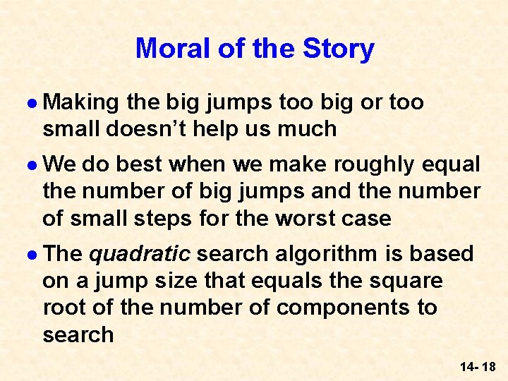
Moral of the Story l Making the big jumps too big or too small doesn’t help us much l We do best when we make roughly equal the number of big jumps and the number of small steps for the worst case l The quadratic search algorithm is based on a jump size that equals the square root of the number of components to search 14 - 18

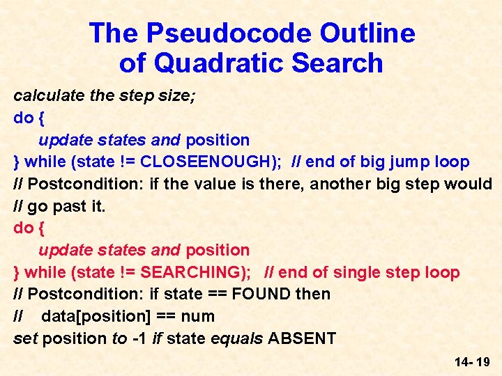
The Pseudocode Outline of Quadratic Search calculate the step size; do { update states and position } while (state != CLOSEENOUGH); // end of big jump loop // Postcondition: if the value is there, another big step would // go past it. do { update states and position } while (state != SEARCHING); // end of single step loop // Postcondition: if state == FOUND then // data[position] == num set position to -1 if state equals ABSENT 14 - 19

int quadratic(int[ ] data, int num) { // Quadratic search through an ordered array. Return -1 for absent num final int FOUND=0, ABSENT=1, SEARCHING=2, CLOSEENOUGH=3; int state = SEARCHING, position = 0, jump. Size; jump. Size = (int) (Math. sqrt(data. length)); do { // by big jumps until we’re close enough if ( (position + jump. Size) >= data. length) state = CLOSEENOUGH; else if (data[position + jump. Size] > num ) state = CLOSEENOUGH; else position = position + jump. Size; } while (state != CLOSEENOUGH); // Postcondition: if num is there, data[position] <= num state = SEARCHING; // reset the current state do { // by single steps until we’re not searching if (position >= data. length) state = ABSENT; else if ( data[position] > num ) state = ABSENT; else if ( data[position] == num ) state = FOUND; else position++; // state is unchanged } while (state == SEARCHING) ; //Postcond. : if num's there, state’s FOUND and data[position] is num } if (state == ABSENT) return -1; else return position; // quadratic

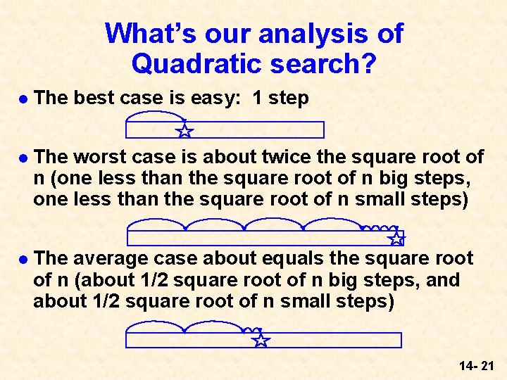
What’s our analysis of Quadratic search? l The best case is easy: 1 step l The worst case is about twice the square root of n (one less than the square root of n big steps, one less than the square root of n small steps) l The average case about equals the square root of n (about 1/2 square root of n big steps, and about 1/2 square root of n small steps) 14 - 21

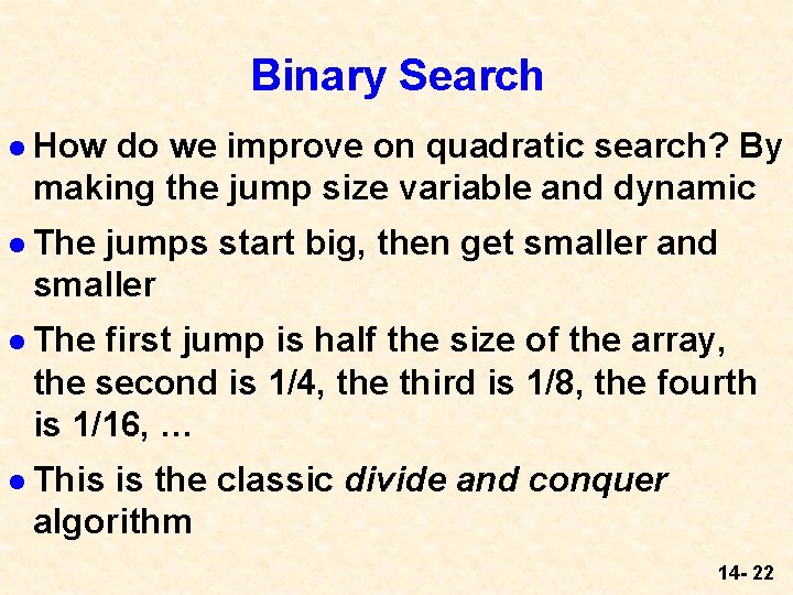
Binary Search l How do we improve on quadratic search? By making the jump size variable and dynamic l The jumps start big, then get smaller and smaller l The first jump is half the size of the array, the second is 1/4, the third is 1/8, the fourth is 1/16, … l This is the classic divide and conquer algorithm 14 - 22

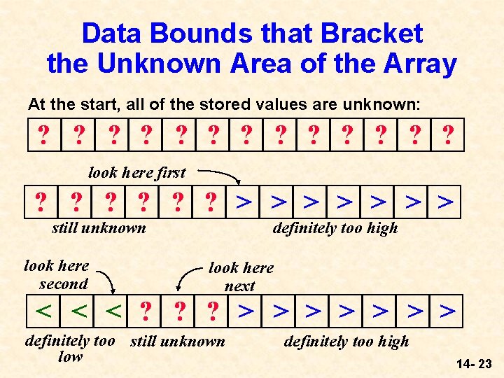
Data Bounds that Bracket the Unknown Area of the Array At the start, all of the stored values are unknown: ? ? ? ? look here first ? ? ? > > > > still unknown look here second definitely too high look here next < < < ? ? ? > > > > definitely too still unknown low definitely too high 14 - 23

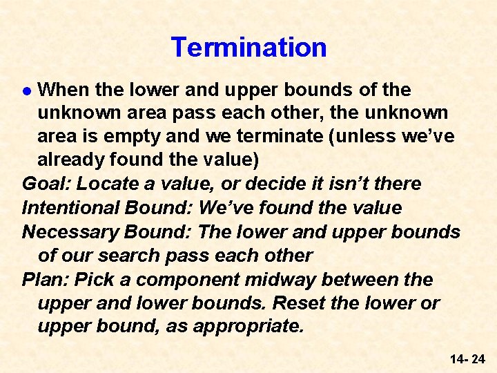
Termination When the lower and upper bounds of the unknown area pass each other, the unknown area is empty and we terminate (unless we’ve already found the value) Goal: Locate a value, or decide it isn’t there Intentional Bound: We’ve found the value Necessary Bound: The lower and upper bounds of our search pass each other Plan: Pick a component midway between the upper and lower bounds. Reset the lower or upper bound, as appropriate. l 14 - 24

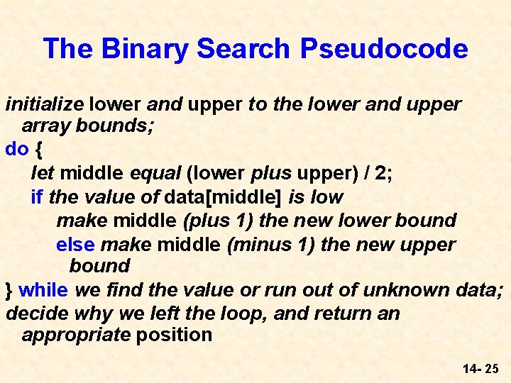
The Binary Search Pseudocode initialize lower and upper to the lower and upper array bounds; do { let middle equal (lower plus upper) / 2; if the value of data[middle] is low make middle (plus 1) the new lower bound else make middle (minus 1) the new upper bound } while we find the value or run out of unknown data; decide why we left the loop, and return an appropriate position 14 - 25

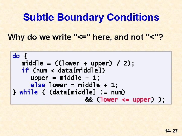
The Binary Search Java Code int binary (int[ ] data, int num) { // Binary search for num in an ordered array int middle, lower = 0, upper = (data. length - 1); do { middle = ((lower + upper) / 2); if (num < data[middle]) upper = middle - 1; else lower = middle + 1; } while ( (data[middle] != num) && (lower <= upper) ); //Postcondition: if data[middle] isn’t num, no // component is if (data[middle] == num) return middle; else return -1; } // binary 14 - 26

Subtle Boundary Conditions Why do we write "<=" here, and not "<"? do { middle = ((lower + upper) / 2); if (num < data[middle]) upper = middle - 1; else lower = middle + 1; } while ( (data[middle] != num) && (lower <= upper) ); 14 - 27

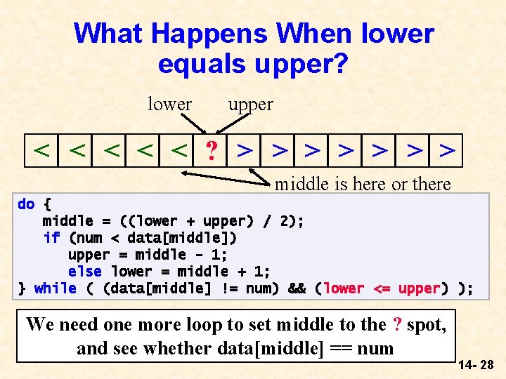
What Happens When lower equals upper? lower upper < < < ? > > > > middle is here or there do { middle = ((lower + upper) / 2); if (num < data[middle]) upper = middle - 1; else lower = middle + 1; } while ( (data[middle] != num) && (lower <= upper) ); We need one more loop to set middle to the ? spot, and see whether data[middle] == num 14 - 28

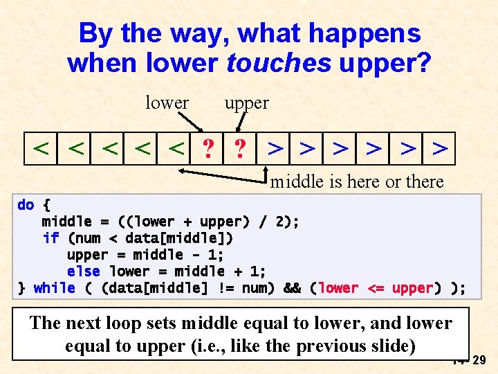
By the way, what happens when lower touches upper? lower upper < < < ? ? > > > middle is here or there do { middle = ((lower + upper) / 2); if (num < data[middle]) upper = middle - 1; else lower = middle + 1; } while ( (data[middle] != num) && (lower <= upper) ); The next loop sets middle equal to lower, and lower equal to upper (i. e. , like the previous slide) 14 - 29

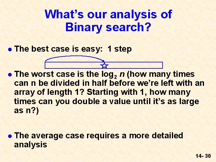
What’s our analysis of Binary search? l The best case is easy: 1 step l The worst case is the log 2 n (how many times can n be divided in half before we’re left with an array of length 1? Starting with 1, how many times can you double a value until it’s as large as n? ) l The average case requires a more detailed analysis 14 - 30

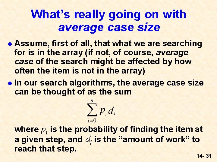
What’s really going on with average case size Assume, first of all, that we are searching for is in the array (if not, of course, average case of the search might be affected by how often the item is not in the array) l In our search algorithms, the average case size can be thought of as the sum l where pi is the probability of finding the item at a given step, and di is the “amount of work” to reach that step. 14 - 31

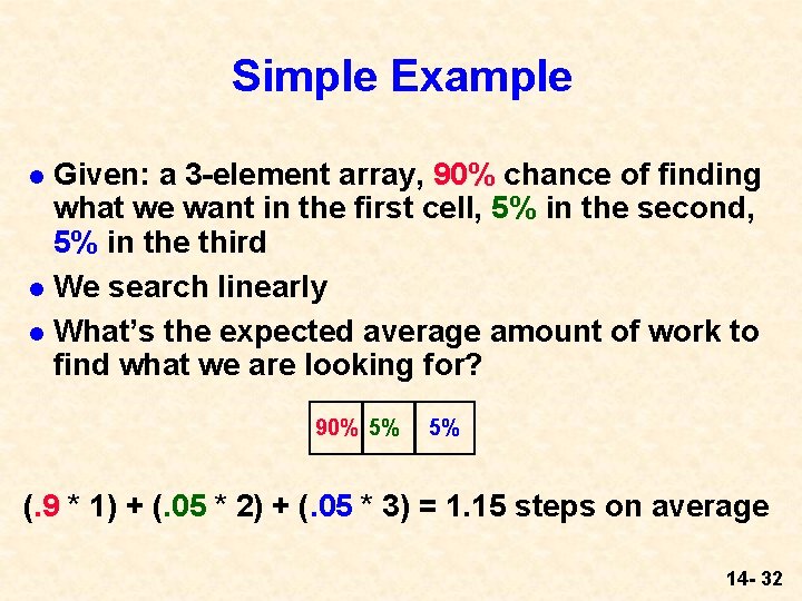
Simple Example Given: a 3 -element array, 90% chance of finding what we want in the first cell, 5% in the second, 5% in the third l We search linearly l What’s the expected average amount of work to find what we are looking for? l 90% 5% 5% (. 9 * 1) + (. 05 * 2) + (. 05 * 3) = 1. 15 steps on average 14 - 32

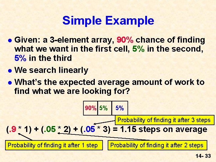
Simple Example Given: a 3 -element array, 90% chance of finding what we want in the first cell, 5% in the second, 5% in the third l We search linearly l What’s the expected average amount of work to find what we are looking for? l 90% 5% 5% Probability of finding it after 3 steps (. 9 * 1) + (. 05 * 2) + (. 05 * 3) = 1. 15 steps on average Probability of finding it after 1 step Probability of finding it after 2 steps 14 - 33

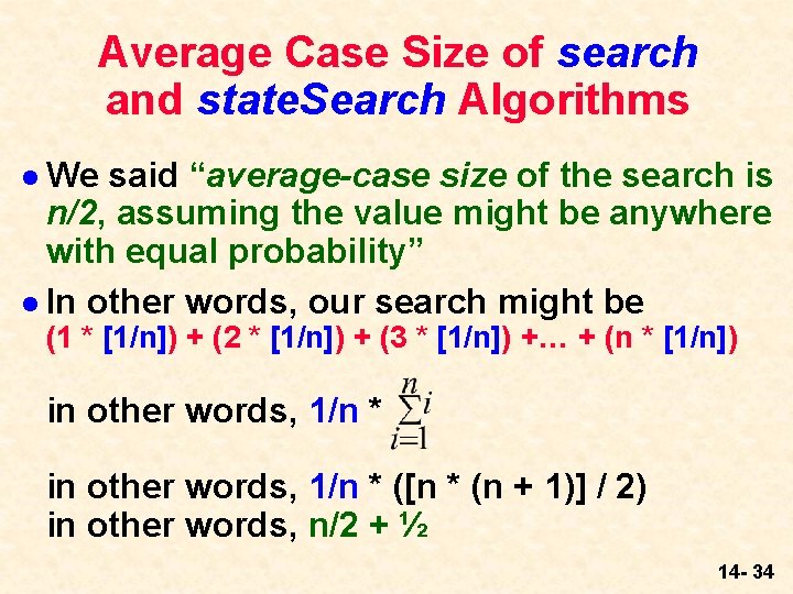
Average Case Size of search and state. Search Algorithms l We said “average-case size of the search is n/2, assuming the value might be anywhere with equal probability” l In other words, our search might be (1 * [1/n]) + (2 * [1/n]) + (3 * [1/n]) +… + (n * [1/n]) in other words, 1/n * ([n * (n + 1)] / 2) in other words, n/2 + ½ 14 - 34

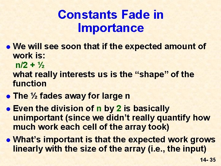
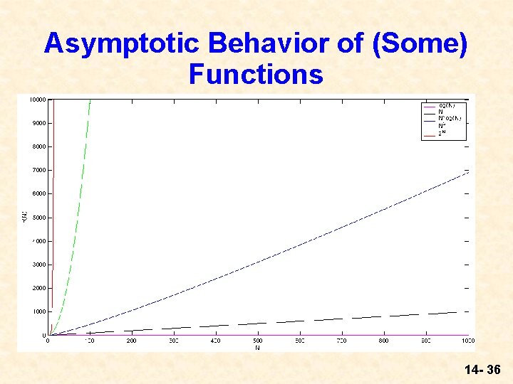
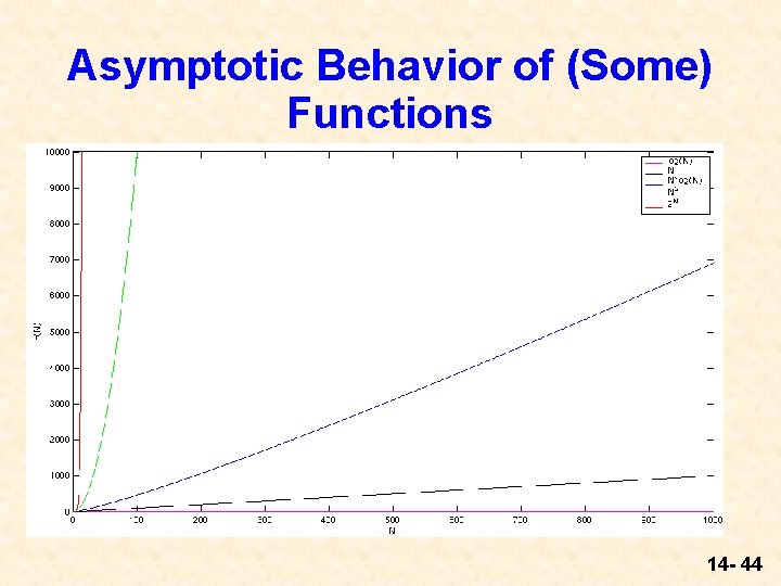
Constants Fade in Importance We will see soon that if the expected amount of work is: n/2 + ½ what really interests us is the “shape” of the function l The ½ fades away for large n l Even the division of n by 2 is basically unimportant (since we didn’t really quantify how much work each cell of the array took) l What’s important is that the expected work grows linearly with the size of the array (i. e. , the input) l 14 - 35

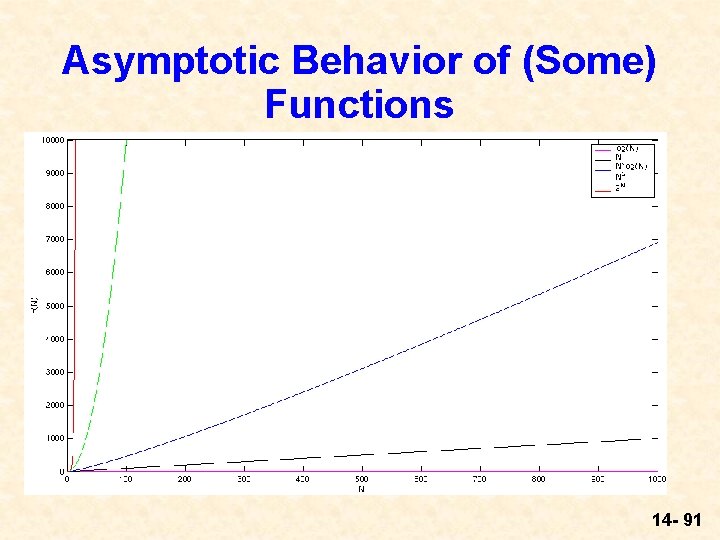
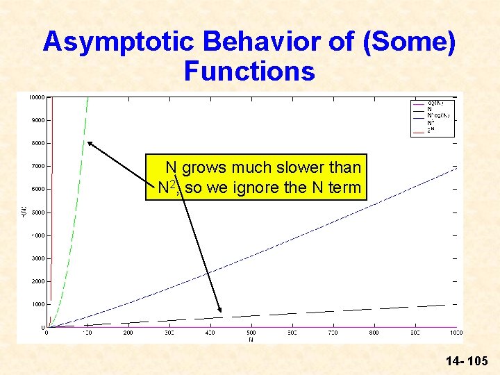
Asymptotic Behavior of (Some) Functions 14 - 36

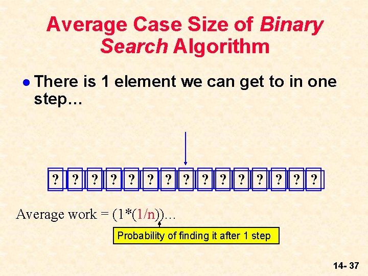
Average Case Size of Binary Search Algorithm l There is 1 element we can get to in one step… ? ? ? ? Average work = (1*(1/n))… Probability of finding it after 1 step 14 - 37

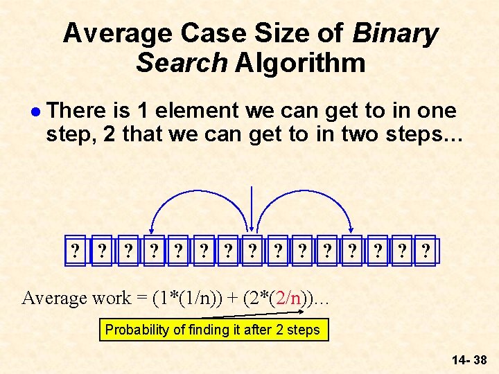
Average Case Size of Binary Search Algorithm l There is 1 element we can get to in one step, 2 that we can get to in two steps… ? ? ? ? Average work = (1*(1/n)) + (2*(2/n))… Probability of finding it after 2 steps 14 - 38

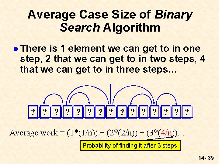
Average Case Size of Binary Search Algorithm l There is 1 element we can get to in one step, 2 that we can get to in two steps, 4 that we can get to in three steps… ? ? ? ? Average work = (1*(1/n)) + (2*(2/n)) + (3*(4/n))… Probability of finding it after 3 steps 14 - 39

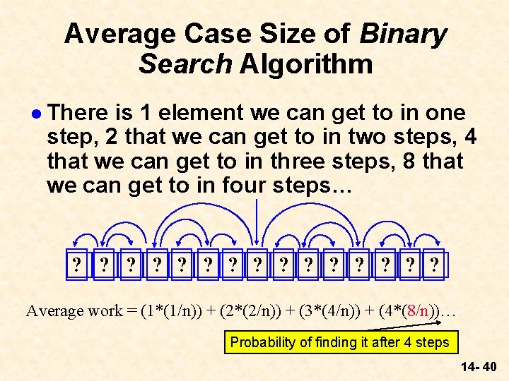
Average Case Size of Binary Search Algorithm l There is 1 element we can get to in one step, 2 that we can get to in two steps, 4 that we can get to in three steps, 8 that we can get to in four steps… ? ? ? ? Average work = (1*(1/n)) + (2*(2/n)) + (3*(4/n)) + (4*(8/n))… Probability of finding it after 4 steps 14 - 40

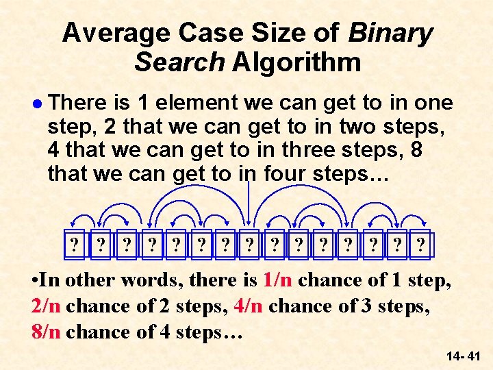
Average Case Size of Binary Search Algorithm l There is 1 element we can get to in one step, 2 that we can get to in two steps, 4 that we can get to in three steps, 8 that we can get to in four steps… ? ? ? ? • In other words, there is 1/n chance of 1 step, 2/n chance of 2 steps, 4/n chance of 3 steps, 8/n chance of 4 steps… 14 - 41

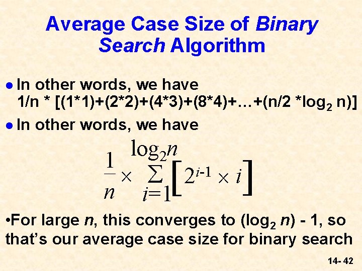
Average Case Size of Binary Search Algorithm l In other words, we have 1/n * [(1*1)+(2*2)+(4*3)+(8*4)+…+(n/2 *log 2 n)] l In other words, we have log 2 n 1 ´ å 2 i-1 ´ i n i=1 [ ] • For large n, this converges to (log 2 n) - 1, so that’s our average case size for binary search 14 - 42

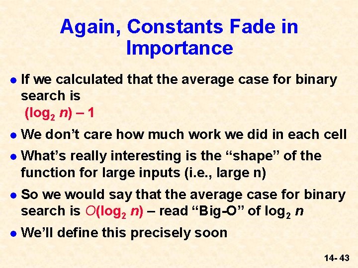
Again, Constants Fade in Importance l If we calculated that the average case for binary search is (log 2 n) – 1 l We don’t care how much work we did in each cell l What’s really interesting is the “shape” of the function for large inputs (i. e. , large n) l So we would say that the average case for binary search is O(log 2 n) – read “Big-O” of log 2 n l We’ll define this precisely soon 14 - 43

Asymptotic Behavior of (Some) Functions 14 - 44

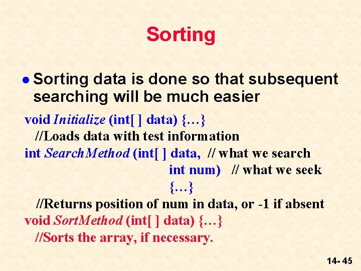
Sorting l Sorting data is done so that subsequent searching will be much easier void Initialize (int[ ] data) {…} //Loads data with test information int Search. Method (int[ ] data, // what we search int num) // what we seek {…} //Returns position of num in data, or -1 if absent void Sort. Method (int[ ] data) {…} //Sorts the array, if necessary. 14 - 45

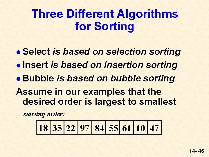
Three Different Algorithms for Sorting l Select is based on selection sorting l Insert is based on insertion sorting l Bubble is based on bubble sorting Assume in our examples that the desired order is largest to smallest starting order: 18 35 22 97 84 55 61 10 47 14 - 46

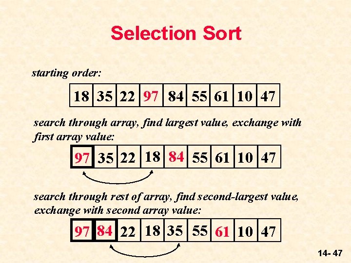
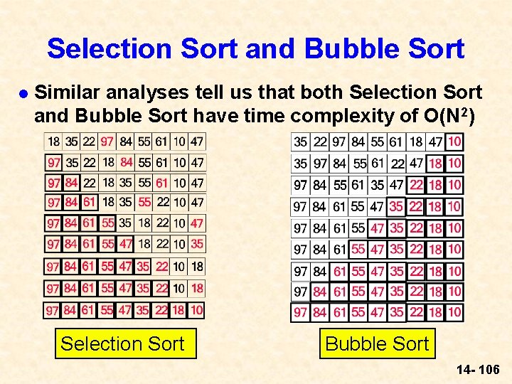
Selection Sort starting order: 18 35 22 97 84 55 61 10 47 search through array, find largest value, exchange with first array value: 97 35 22 18 84 55 61 10 47 search through rest of array, find second-largest value, exchange with second array value: 97 84 22 18 35 55 61 10 47 14 - 47

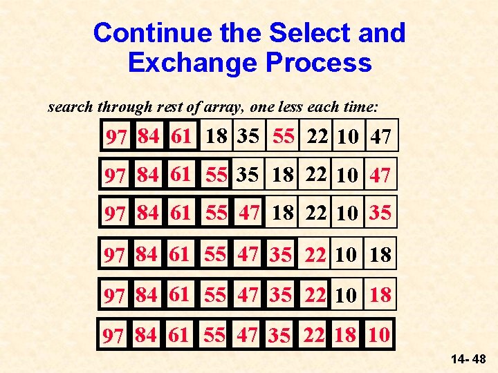
Continue the Select and Exchange Process search through rest of array, one less each time: 97 84 61 18 35 55 22 10 47 97 84 61 55 35 18 22 10 47 97 84 61 55 47 18 22 10 35 97 84 61 55 47 35 22 10 18 97 84 61 55 47 35 22 18 10 14 - 48

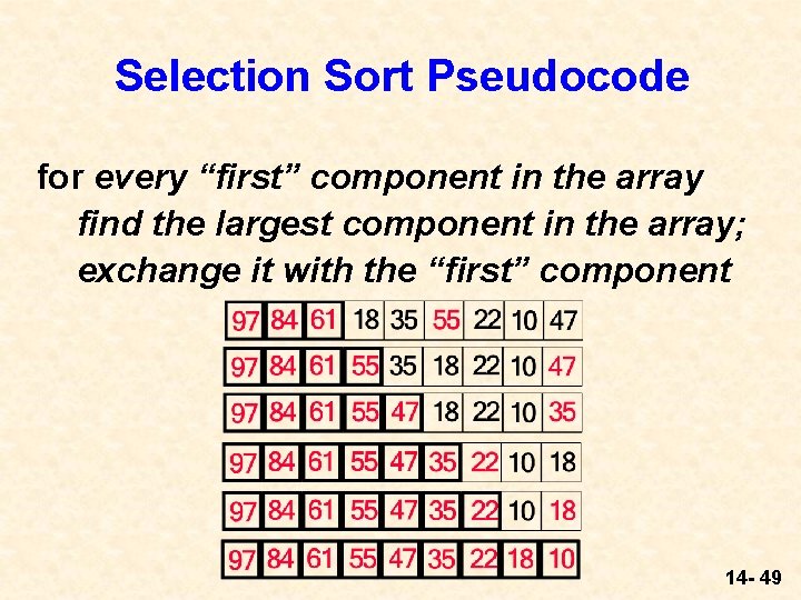
Selection Sort Pseudocode for every “first” component in the array find the largest component in the array; exchange it with the “first” component 14 - 49

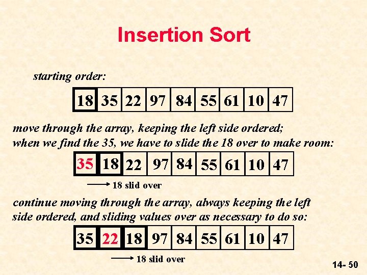
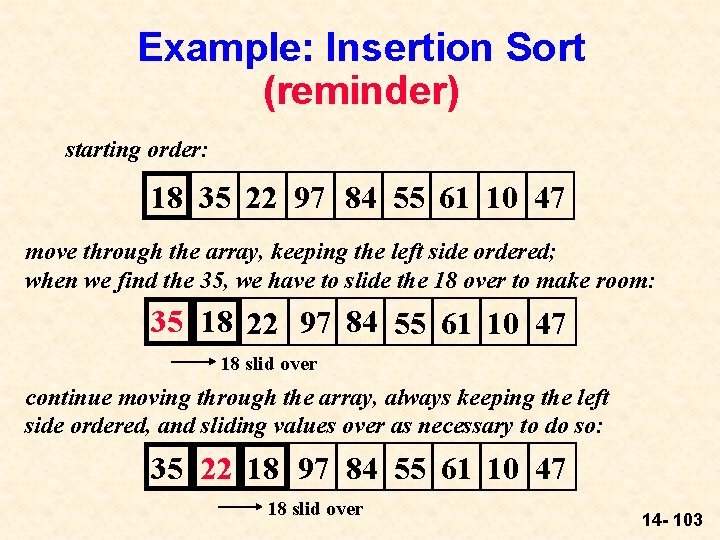
Insertion Sort starting order: 18 35 22 97 84 55 61 10 47 move through the array, keeping the left side ordered; when we find the 35, we have to slide the 18 over to make room: 35 18 22 97 84 55 61 10 47 18 slid over continue moving through the array, always keeping the left side ordered, and sliding values over as necessary to do so: 35 22 18 97 84 55 61 10 47 18 slid over 14 - 50

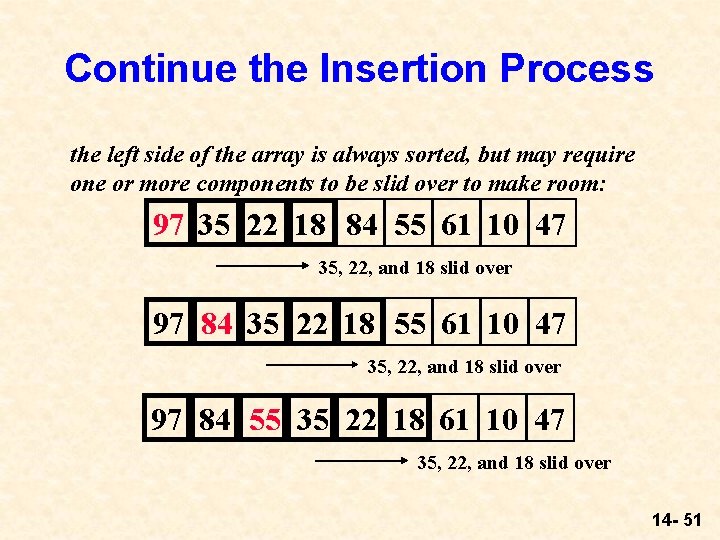
Continue the Insertion Process the left side of the array is always sorted, but may require one or more components to be slid over to make room: 97 35 22 18 84 55 61 10 47 35, 22, and 18 slid over 97 84 35 22 18 55 61 10 47 35, 22, and 18 slid over 97 84 55 35 22 18 61 10 47 35, 22, and 18 slid over 14 - 51

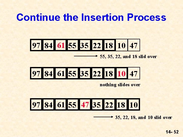
Continue the Insertion Process 97 84 61 55 35 22 18 10 47 55, 35, 22, and 18 slid over 97 84 61 55 35 22 18 10 47 nothing slides over 97 84 61 55 47 35 22 18 10 35, 22, 18, and 10 slid over 14 - 52

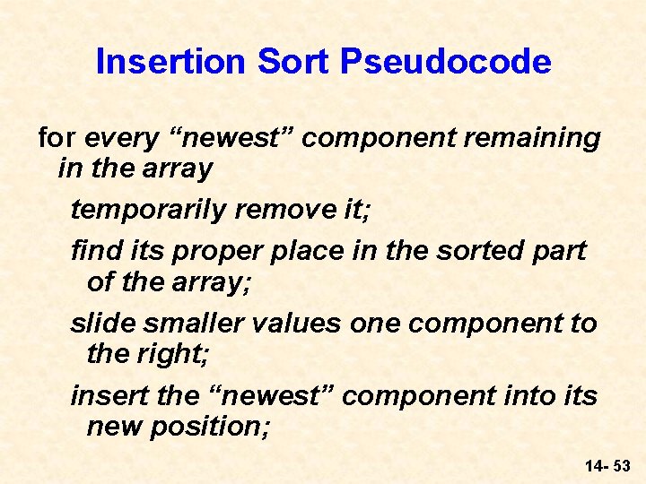
Insertion Sort Pseudocode for every “newest” component remaining in the array temporarily remove it; find its proper place in the sorted part of the array; slide smaller values one component to the right; insert the “newest” component into its new position; 14 - 53

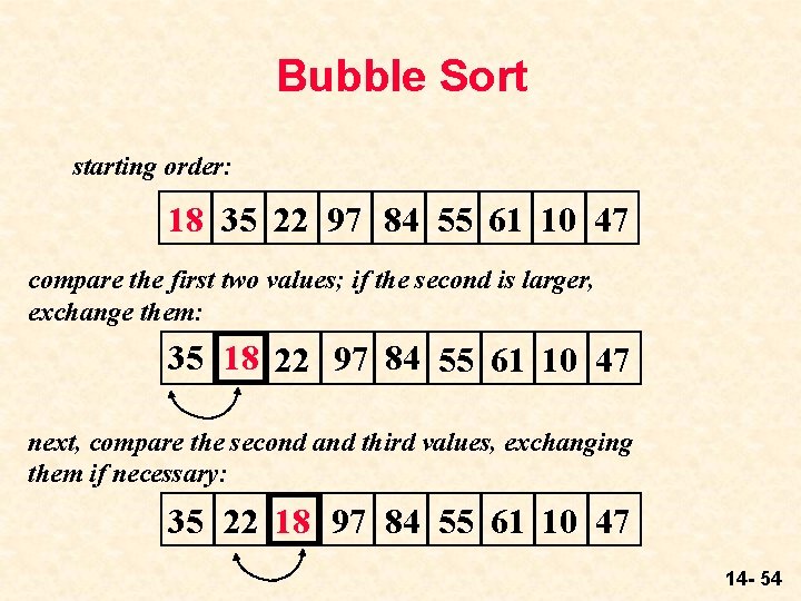
Bubble Sort starting order: 18 35 22 97 84 55 61 10 47 compare the first two values; if the second is larger, exchange them: 35 18 22 97 84 55 61 10 47 next, compare the second and third values, exchanging them if necessary: 35 22 18 97 84 55 61 10 47 14 - 54

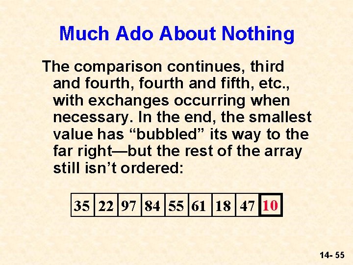
Much Ado About Nothing The comparison continues, third and fourth, fourth and fifth, etc. , with exchanges occurring when necessary. In the end, the smallest value has “bubbled” its way to the far right—but the rest of the array still isn’t ordered: 35 22 97 84 55 61 18 47 10 14 - 55

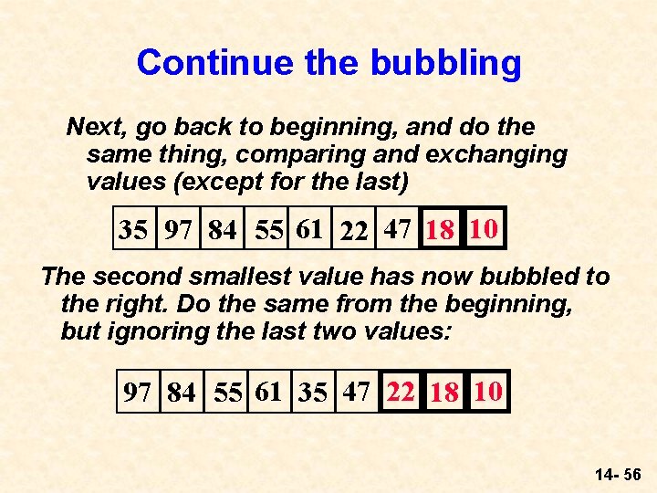
Continue the bubbling Next, go back to beginning, and do the same thing, comparing and exchanging values (except for the last) 35 97 84 55 61 22 47 18 10 The second smallest value has now bubbled to the right. Do the same from the beginning, but ignoring the last two values: 97 84 55 61 35 47 22 18 10 14 - 56

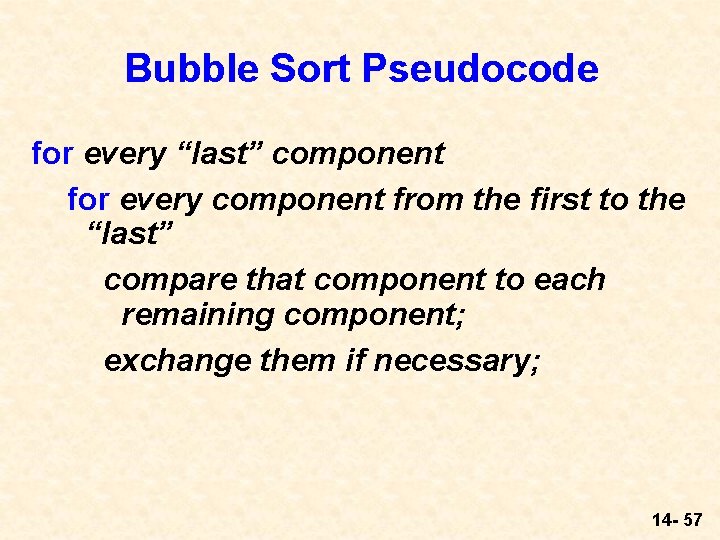
Bubble Sort Pseudocode for every “last” component for every component from the first to the “last” compare that component to each remaining component; exchange them if necessary; 14 - 57

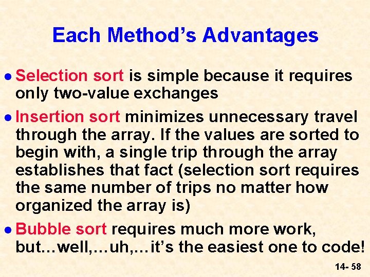
Each Method’s Advantages l Selection sort is simple because it requires only two-value exchanges l Insertion sort minimizes unnecessary travel through the array. If the values are sorted to begin with, a single trip through the array establishes that fact (selection sort requires the same number of trips no matter how organized the array is) l Bubble sort requires much more work, but…well, …uh, …it’s the easiest one to code! 14 - 58

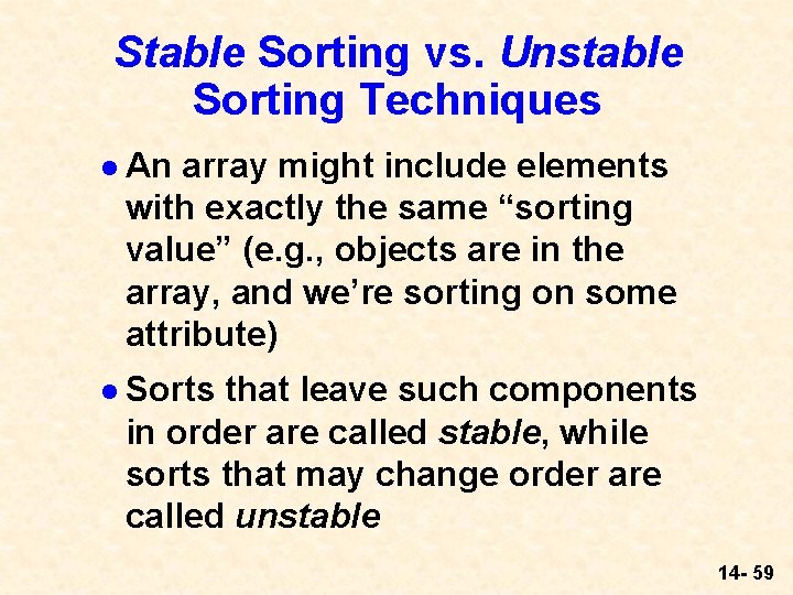
Stable Sorting vs. Unstable Sorting Techniques l An array might include elements with exactly the same “sorting value” (e. g. , objects are in the array, and we’re sorting on some attribute) l Sorts that leave such components in order are called stable, while sorts that may change order are called unstable 14 - 59

The Selection Sort Java Code void select (int[ ] data) { // Uses selection sort to order an array of integers. int first, current, largest, temp; for (first = 0; first < data. length - 1; first++) { largest = first; for (current = first + 1; current < data. length; current++) { if ( data[current] > data[largest] ) largest = current; } // Postcondition: largest is index of largest item // from first. . end of array if (largest != first) { // We have to make a swap temp = data[largest]; data[largest] = data[first]; // Make the swap data[first] = temp; } } } // select 14 - 60

The Insertion Sort Java Code void insert (int[ ] data) { // Uses insertion sort to order an array of integers. int newest, current, new. Item; boolean seeking; for (newest = 1; newest < data. length; newest++) { seeking = true; current = newest; new. Item = data[newest]; while (seeking) { // seeking new. Item's new position on left if (data[current - 1] < new. Item) { data[current] = data[current -1]; //slide value right current--; seeking = (current > 0); } else seeking = false; } // while // Postcondition: new. Item belongs in data[current] = new. Item; } // newest for } // insert 14 - 61

The Bubble Sort Java Code void bubble (int[ ] data) { // Uses bubble sort to order an array of integers. int last, current, temp; for (last = data. length-1; last > 0; last--) { for (current = 0; current < last; current++) { if ( data[current] < data[current + 1] ) { temp = data[current]; data[current] = data[current + 1]; data[current + 1] = temp; } // if } // current for //Postcondition: Components last through the end of // the array are ordered. } // last for } // bubble 14 - 62

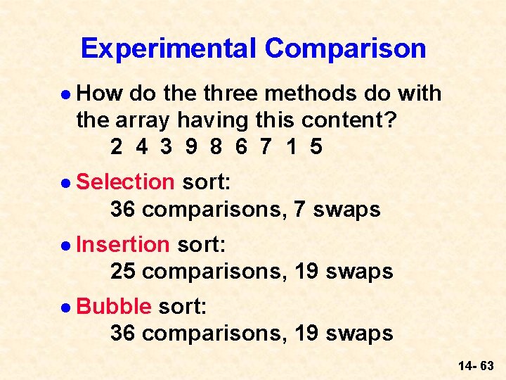
Experimental Comparison l How do the three methods do with the array having this content? 2 4 3 9 8 6 7 1 5 l Selection sort: 36 comparisons, 7 swaps l Insertion sort: 25 comparisons, 19 swaps l Bubble sort: 36 comparisons, 19 swaps 14 - 63

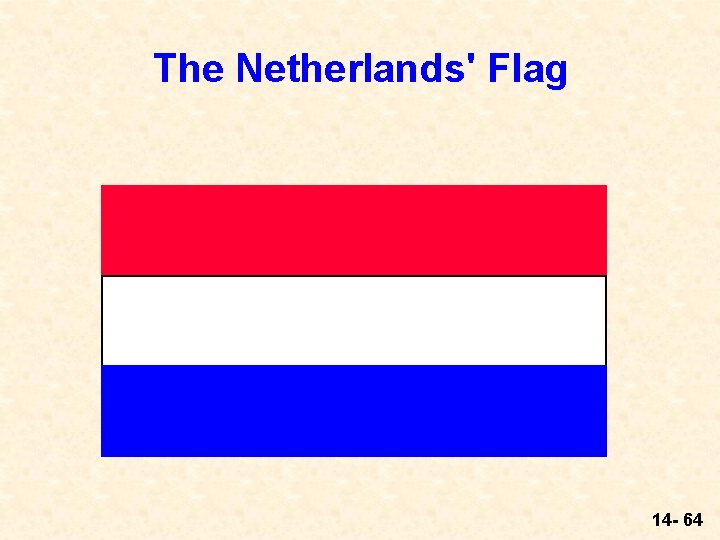
The Netherlands' Flag 14 - 64

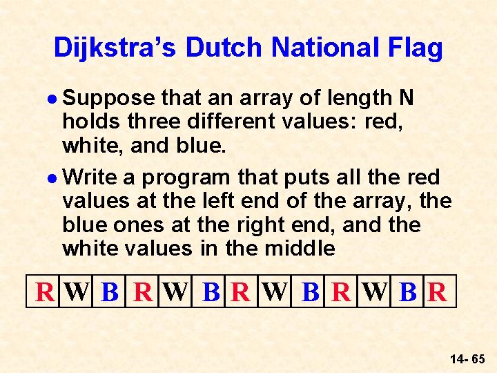
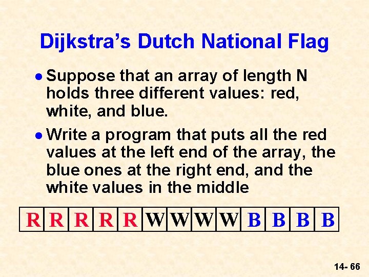
Dijkstra’s Dutch National Flag l Suppose that an array of length N holds three different values: red, white, and blue. l Write a program that puts all the red values at the left end of the array, the blue ones at the right end, and the white values in the middle RWB RWB R 14 - 65

Dijkstra’s Dutch National Flag l Suppose that an array of length N holds three different values: red, white, and blue. l Write a program that puts all the red values at the left end of the array, the blue ones at the right end, and the white values in the middle R R R WWW W B B 14 - 66

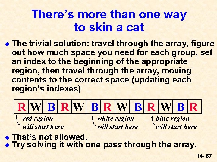
There’s more than one way to skin a cat l The trivial solution: travel through the array, figure out how much space you need for each group, set an index to the beginning of the appropriate region, then travel through the array, moving contents to the correct space (updating each region’s indexes) RW B RWB R red region will start here l l white region will start here blue region will start here That’s not allowed. Try solving it with one pass through the array. 14 - 67

Why we’re doing this l The solution provides a good example of using a bunch of our previous techniques: usubscripts into an array as indexes ucase analysis to guide the decisionmaking in the algorithm uusing data bounds to decide when to leave a loop ualso uses some ideas from our “sorting/searching” programs 14 - 68

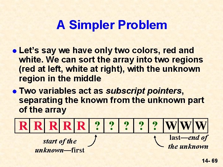
A Simpler Problem Let’s say we have only two colors, red and white. We can sort the array into two regions (red at left, white at right), with the unknown region in the middle l Two variables act as subscript pointers, separating the known from the unknown part of the array l R R R ? ? ? WW W start of the unknown—first last—end of the unknown 14 - 69

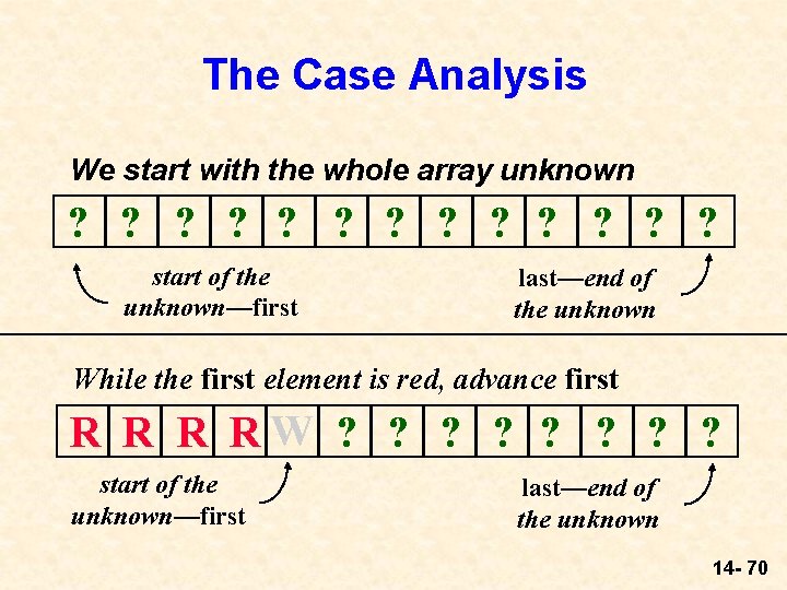
The Case Analysis We start with the whole array unknown ? ? ? ? start of the unknown—first last—end of the unknown While the first element is red, advance first R RW ? ? ? ? start of the unknown—first last—end of the unknown 14 - 70

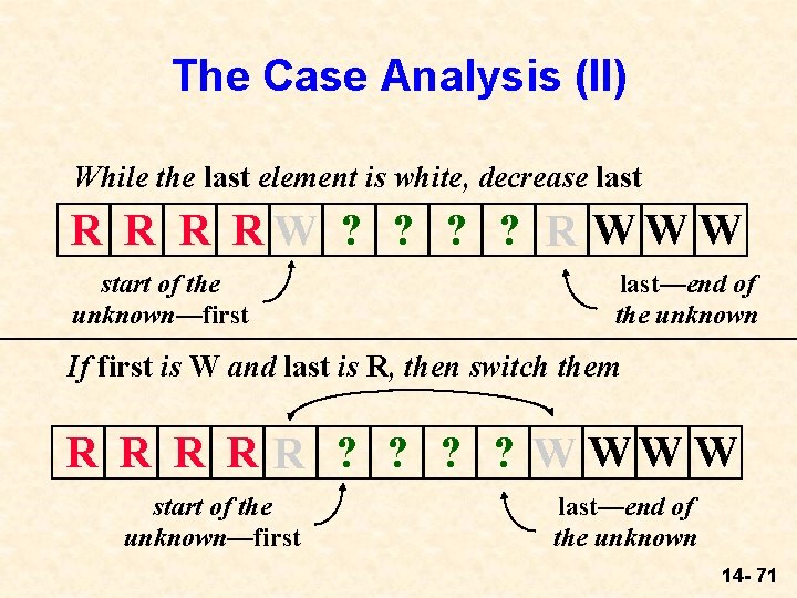
The Case Analysis (II) While the last element is white, decrease last R R W ? ? R WW W start of the unknown—first last—end of the unknown If first is W and last is R, then switch them R R R ? ? W WW W start of the unknown—first last—end of the unknown 14 - 71

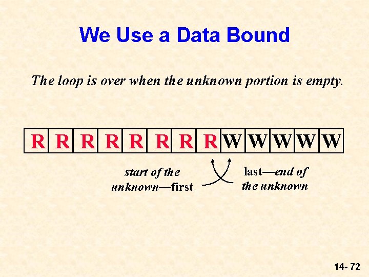
We Use a Data Bound The loop is over when the unknown portion is empty. R R R RW WWW W start of the unknown—first last—end of the unknown 14 - 72

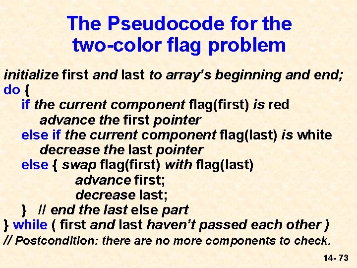
The Pseudocode for the two-color flag problem initialize first and last to array’s beginning and end; do { if the current component flag(first) is red advance the first pointer else if the current component flag(last) is white decrease the last pointer else { swap flag(first) with flag(last) advance first; decrease last; } // end the last else part } while ( first and last haven’t passed each other ) // Postcondition: there are no more components to check. 14 - 73

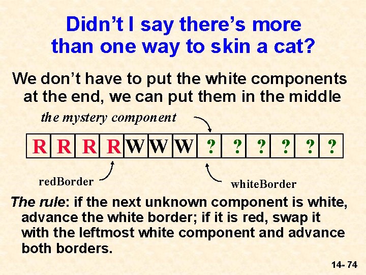
Didn’t I say there’s more than one way to skin a cat? We don’t have to put the white components at the end, we can put them in the middle the mystery component R RWW W ? ? ? red. Border white. Border The rule: if the next unknown component is white, advance the white border; if it is red, swap it with the leftmost white component and advance both borders. 14 - 74

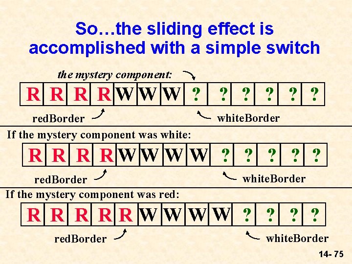
So…the sliding effect is accomplished with a simple switch the mystery component: R RWW W ? ? ? red. Border If the mystery component was white: white. Border R RWW W W ? ? ? red. Border If the mystery component was red: white. Border R R RWWWW ? ? red. Border white. Border 14 - 75

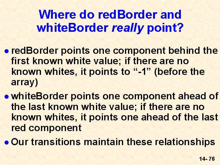
Where do red. Border and white. Border really point? l red. Border points one component behind the first known white value; if there are no known whites, it points to “-1” (before the array) l white. Border points one component ahead of the last known white value; if there are no known whites, it points one ahead of the last red component l Our transitions maintain these relationships 14 - 76

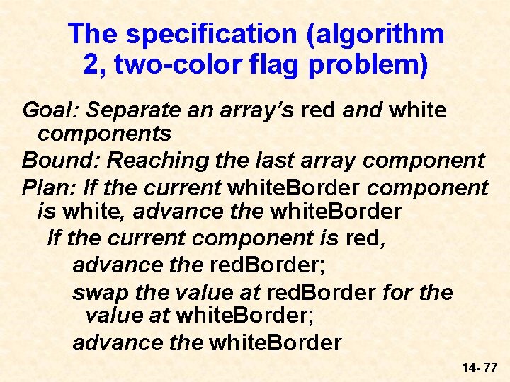
The specification (algorithm 2, two-color flag problem) Goal: Separate an array’s red and white components Bound: Reaching the last array component Plan: If the current white. Border component is white, advance the white. Border If the current component is red, advance the red. Border; swap the value at red. Border for the value at white. Border; advance the white. Border 14 - 77

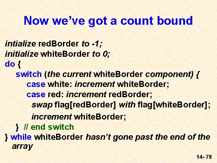
Now we’ve got a count bound intialize red. Border to -1; initialize white. Border to 0; do { switch (the current white. Border component) { case white: increment white. Border; case red: increment red. Border; swap flag[red. Border] with flag[white. Border]; increment white. Border; } // end switch } while white. Border hasn’t gone past the end of the array 14 - 78

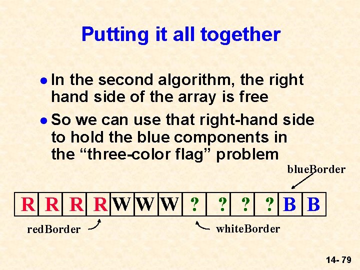
Putting it all together l In the second algorithm, the right hand side of the array is free l So we can use that right-hand side to hold the blue components in the “three-color flag” problem blue. Border R RWW W ? ? B B red. Border white. Border 14 - 79

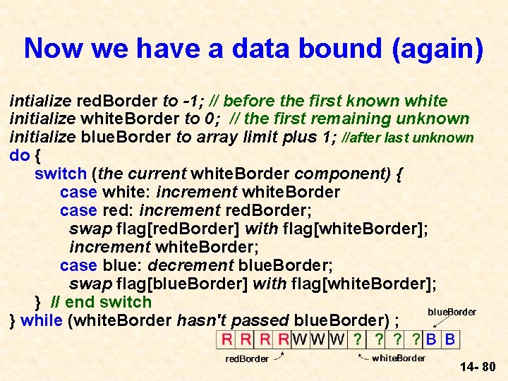
Now we have a data bound (again) intialize red. Border to -1; // before the first known white initialize white. Border to 0; // the first remaining unknown initialize blue. Border to array limit plus 1; //after last unknown do { switch (the current white. Border component) { case white: increment white. Border case red: increment red. Border; swap flag[red. Border] with flag[white. Border]; increment white. Border; case blue: decrement blue. Border; swap flag[blue. Border] with flag[white. Border]; } // end switch } while (white. Border hasn't passed blue. Border) ; 14 - 80

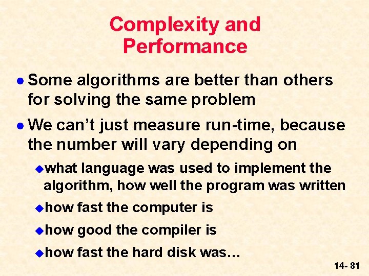
Complexity and Performance l Some algorithms are better than others for solving the same problem l We can’t just measure run-time, because the number will vary depending on uwhat language was used to implement the algorithm, how well the program was written uhow fast the computer is uhow good the compiler is uhow fast the hard disk was… 14 - 81

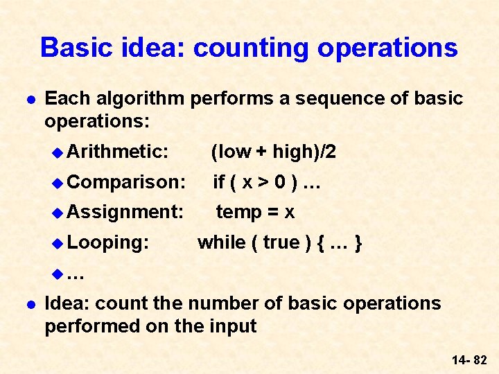
Basic idea: counting operations l Each algorithm performs a sequence of basic operations: u Arithmetic: (low + high)/2 u Comparison: if ( x > 0 ) … u Assignment: temp = x u Looping: while ( true ) { … } u… l Idea: count the number of basic operations performed on the input 14 - 82

It Depends l Difficulties: u. Which operations are basic? u. Not all operations take the same amount of time u. Operations take different times with different hardware or compilers 14 - 83

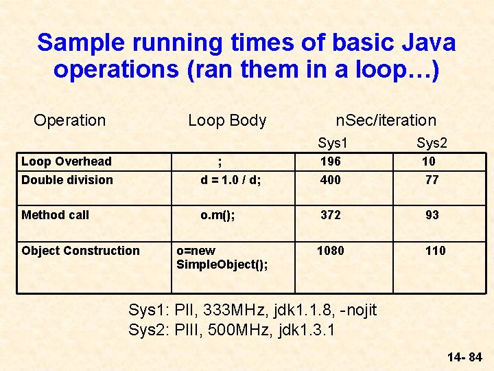
Sample running times of basic Java operations (ran them in a loop…) Operation Loop Body n. Sec/iteration Sys 1 Sys 2 Loop Overhead Double division ; d = 1. 0 / d; 196 400 10 77 Method call o. m(); 372 93 1080 110 Object Construction o=new Simple. Object(); Sys 1: PII, 333 MHz, jdk 1. 1. 8, -nojit Sys 2: PIII, 500 MHz, jdk 1. 3. 1 14 - 84

So instead… l We use mathematical functions that estimate or bound: uthe growth rate of a problem’s difficulty, or uthe performance of an algorithm l Our Motivation: analyze the running time of an algorithm as a function of only simple parameters of the input 14 - 85

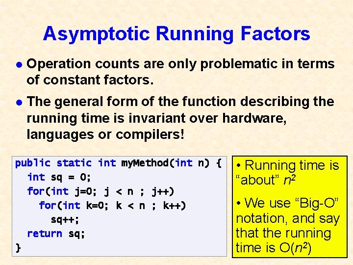
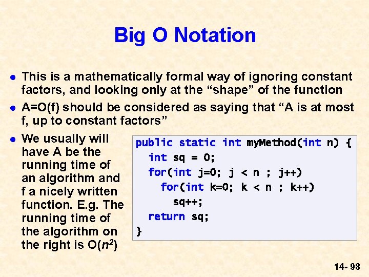
Asymptotic Running Factors l Operation counts are only problematic in terms of constant factors. l The general form of the function describing the running time is invariant over hardware, languages or compilers! public static int my. Method(int n) { int sq = 0; for(int j=0; j < n ; j++) for(int k=0; k < n ; k++) sq++; return sq; } • Running time is “about” n 2 • We use “Big-O” notation, and say that the running time is O(n 2) 14 - 86

The Problem’s Size l The problem’s size is stated in terms of n, which might be: uthe number of components in an array uthe number of items in a file uthe number of pixels on a screen uthe amount of output the program is expected to produce 14 - 87

Example l Linear growth in complexity (searching an array, one component after another, to find an element): time to perform the search n number of components 14 - 88

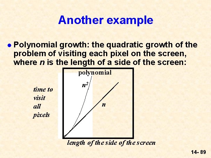
Another example l Polynomial growth: the quadratic growth of the problem of visiting each pixel on the screen, where n is the length of a side of the screen: polynomial time to visit all pixels n 2 n length of the side of the screen 14 - 89

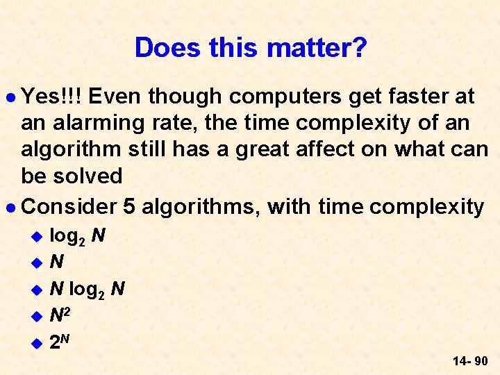
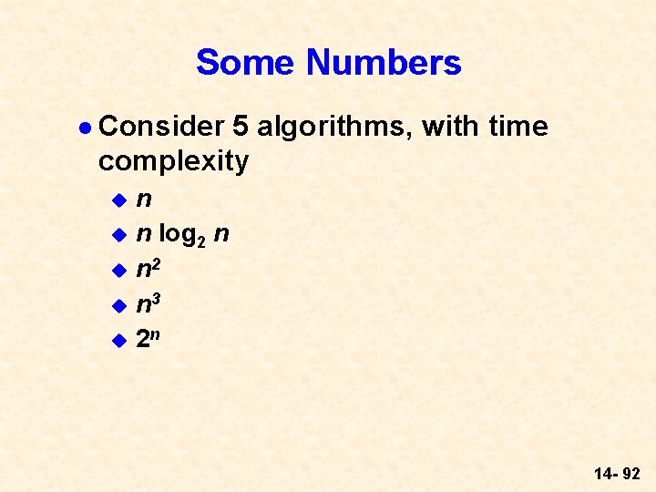
Does this matter? l Yes!!! Even though computers get faster at an alarming rate, the time complexity of an algorithm still has a great affect on what can be solved l Consider 5 algorithms, with time complexity log 2 N u N log 2 N u N 2 u 2 N u 14 - 90

Asymptotic Behavior of (Some) Functions 14 - 91

Some Numbers l Consider 5 algorithms, with time complexity n u n log 2 n u n 2 u n 3 u 2 n u 14 - 92

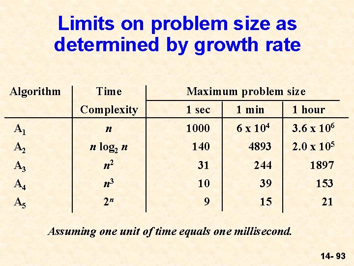
Limits on problem size as determined by growth rate Algorithm Time Maximum problem size Complexity 1 sec 1 min 1 hour A 1 n 1000 6 x 104 3. 6 x 106 A 2 n log 2 n 140 4893 2. 0 x 105 A 3 n 2 31 244 1897 A 4 n 3 10 39 153 A 5 2 n 9 15 21 Assuming one unit of time equals one millisecond. 14 - 93

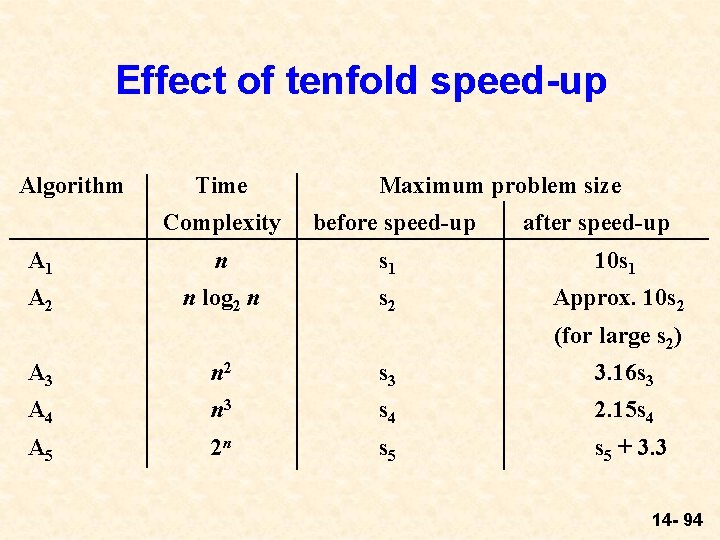
Effect of tenfold speed-up Algorithm Time Maximum problem size Complexity before speed-up after speed-up A 1 n s 1 10 s 1 A 2 n log 2 n s 2 Approx. 10 s 2 (for large s 2) A 3 n 2 s 3 3. 16 s 3 A 4 n 3 s 4 2. 15 s 4 A 5 2 n s 5 + 3. 3 14 - 94

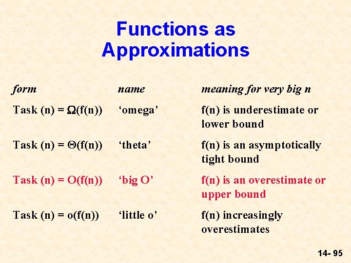
Functions as Approximations form name meaning for very big n Task (n) = (f(n)) ‘omega’ f(n) is underestimate or lower bound Task (n) = Θ(f(n)) ‘theta’ f(n) is an asymptotically tight bound Task (n) = O(f(n)) ‘big O’ f(n) is an overestimate or upper bound Task (n) = o(f(n)) ‘little o’ f(n) increasingly overestimates 14 - 95

Big O Notation l Big O notation is the most useful for us; it says that a function f(n) serves as an upper bound on real-life performance. l For algorithm A of size n (informally): The complexity of A(n) is on the order of f(n) if A(n) is less than or equal to some constant times f(n) l The constant can be anything as long as the relation holds once n reaches some threshold. 14 - 96

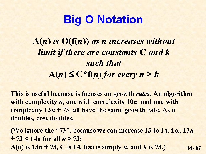
Big O Notation A(n) is O(f(n)) as n increases without limit if there are constants C and k such that A(n) C*f(n) for every n > k This is useful because is focuses on growth rates. An algorithm with complexity n, one with complexity 10 n, and one with complexity 13 n + 73, all have the same growth rate. As n doubles, cost doubles. (We ignore the “ 73”, because we can increase 13 to 14, i. e. , 13 n + 73 14 n for all n 73; A(n) is 13 n + 73, C is 14, f(n) is simply n, and k is 73. ) 14 - 97

Big O Notation l l l This is a mathematically formal way of ignoring constant factors, and looking only at the “shape” of the function A=O(f) should be considered as saying that “A is at most f, up to constant factors” We usually will public static int my. Method(int n) { have A be the int sq = 0; running time of for(int j=0; j < n ; j++) an algorithm and for(int k=0; k < n ; k++) f a nicely written sq++; function. E. g. The return sq; running time of the algorithm on } the right is O(n 2) 14 - 98

Asymptotic Analysis of Algorithms l l l We usually embark on an asymptotic worst case analysis of the running time of the algorithm. Asymptotic: u Formal, exact, depends only on the algorithm u Ignores constants u Applicable mostly for large input sizes Worst Case: u Bounds on running time must hold for all inputs u Thus the analysis considers the worst-case input u Sometimes the “average” performance can be much better u Real-life inputs rarely “average” in any formal sense 14 - 99

Worst Case/Best Case l Worst case performance measure of an algorithm states an upper bound l Best case complexity measure of a problem states a lower bound; no algorithm can take less time 14 - 100

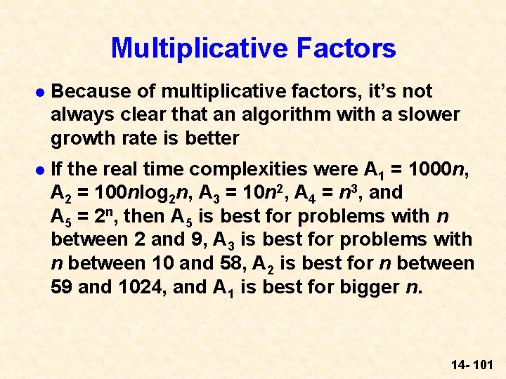
Multiplicative Factors l Because of multiplicative factors, it’s not always clear that an algorithm with a slower growth rate is better l If the real time complexities were A 1 = 1000 n, A 2 = 100 nlog 2 n, A 3 = 10 n 2, A 4 = n 3, and A 5 = 2 n, then A 5 is best for problems with n between 2 and 9, A 3 is best for problems with n between 10 and 58, A 2 is best for n between 59 and 1024, and A 1 is best for bigger n. 14 - 101

An Example: Binary Search l Binary search splits the unknown portion of the array in half; the worst-case search will be O(log 2 n) l Doubling n only increases the logarithm by 1; growth is very slow 14 - 102

Example: Insertion Sort (reminder) starting order: 18 35 22 97 84 55 61 10 47 move through the array, keeping the left side ordered; when we find the 35, we have to slide the 18 over to make room: 35 18 22 97 84 55 61 10 47 18 slid over continue moving through the array, always keeping the left side ordered, and sliding values over as necessary to do so: 35 22 18 97 84 55 61 10 47 18 slid over 14 - 103

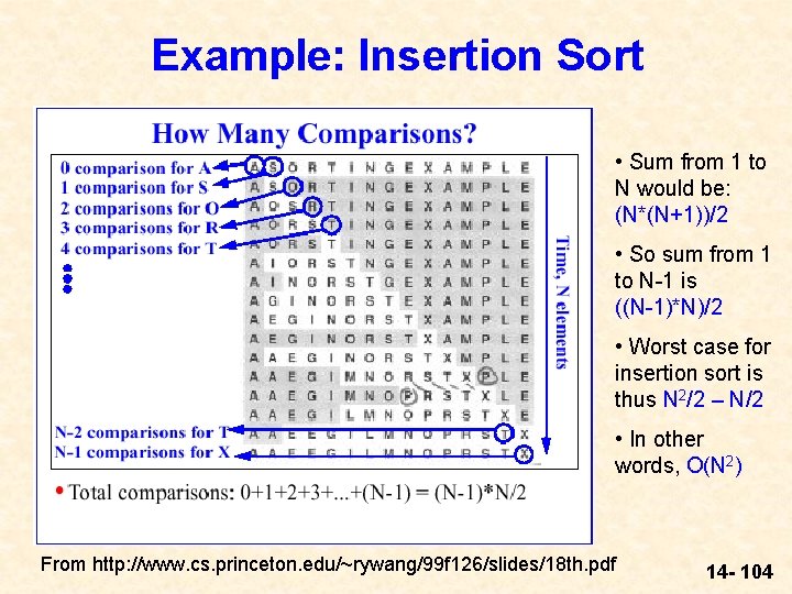
Example: Insertion Sort • Sum from 1 to N would be: (N*(N+1))/2 • So sum from 1 to N-1 is ((N-1)*N)/2 • Worst case for insertion sort is thus N 2/2 – N/2 • In other words, O(N 2) From http: //www. cs. princeton. edu/~rywang/99 f 126/slides/18 th. pdf 14 - 104

Asymptotic Behavior of (Some) Functions N grows much slower than N 2, so we ignore the N term 14 - 105

Selection Sort and Bubble Sort l Similar analyses tell us that both Selection Sort and Bubble Sort have time complexity of O(N 2) Selection Sort Bubble Sort 14 - 106

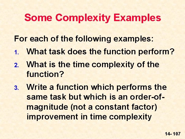
Some Complexity Examples For each of the following examples: 1. What task does the function perform? 2. What is the time complexity of the function? 3. Write a function which performs the same task but which is an order-ofmagnitude (not a constant factor) improvement in time complexity 14 - 107

Example 1 public int some. Method 1 (int[] a) { int temp = 0; for (int i=0; i < a. length; i++) for (int j=i+1; j < a. length; j++) if (Math. abs(a[j]-a[i]) > temp) temp = Math. abs(a[j]-a[i]); return temp; } 14 - 108

Example 1 public int some. Method 1 (int[] a) { int temp = 0; for (int i=0; i < a. length; i++) for (int j=i+1; j < a. length; j++) if (Math. abs(a[j]-a[i]) > temp) temp = Math. abs(a[j]-a[i]); return temp; } 1. Finds maximum difference between two values in the array 14 - 109

Example 1 public int some. Method 1 (int[] a) { int temp = 0; for (int i=0; i < a. length; i++) for (int j=i+1; j < a. length; j++) if (Math. abs(a[j]-a[i]) > temp) temp = Math. abs(a[j]-a[i]); return temp; } 1. Finds maximum difference between two values in the array 2. O(n 2) 14 - 110

Example 1 public int some. Method 1 (int[] a) { int temp = 0; for (int i=0; i < a. length; i++) for (int j=i+1; j < a. length; j++) if (Math. abs(a[j]-a[i]) > temp) temp = Math. abs(a[j]-a[i]); return temp; } 1. Finds maximum difference between two values in the array 2. O(n 2) 3. Find the max and min values in the array, then subtract one from the other – the problem will be solved in O(n) 14 - 111

Example 2: a[ ] is sorted in increasing order, b[ ] is not sorted public boolean some. Method 2(int[] a, int[] b) { for (int j=0; j < b. length; j++) for (int i=0; i < a. length-1; i++) if (b[j] == a[i] + a[i+1]) return true; return false; } 14 - 112

Example 2: a[ ] is sorted in increasing order, b[ ] is not sorted public boolean some. Method 2(int[] a, int[] b) { for (int j=0; j < b. length; j++) for (int i=0; i < a. length-1; i++) if (b[j] == a[i] + a[i+1]) return true; return false; } 1. Checks whether a value in b[ ] equals the sum of two consecutive values in a[ ] 14 - 113

Example 2: a[ ] is sorted in increasing order, b[ ] is not sorted public boolean some. Method 2(int[] a, int[] b) { for (int j=0; j < b. length; j++) for (int i=0; i < a. length-1; i++) if (b[j] == a[i] + a[i+1]) return true; return false; } 1. Checks whether a value in b[ ] equals the sum of two consecutive values in a[ ] 2. O(n 2) 14 - 114

Example 2: a[ ] is sorted in increasing order, b[ ] is not sorted public boolean some. Method 2(int[] a, int[] b) { for (int j=0; j < b. length; j++) for (int i=0; i < a. length-1; i++) if (b[j] == a[i] + a[i+1]) return true; return false; } 1. Checks whether a value in b[ ] equals the sum of two consecutive values in a[ ] 2. O(n 2) 3. For each value in b[ ], carry out a variation of a binary search in a[ ] – the problem will be solved in O(n log n) 14 - 115

Example 3: each element of a[ ] is a unique int between 1 and n; a. length is n-1 public int some. Method 3 (int[] a) { boolean flag; for (int j=1; j<=a. length+1; j++) { flag = false; for (int i=0; i<a. length; i++) { if (a[i]==j) { flag = true; break; } } if (!flag) return j; } return -1; } 14 - 116

Example 3: each element of a[ ] is a unique int between 1 and n; a. length is n-1 public int some. Method 3 (int[] a) { boolean flag; for (int j=1; j<=a. length+1; j++) { flag = false; for (int i=0; i<a. length; i++) { if (a[i]==j) { flag = true; break; } } if (!flag) return j; } return -1; } 1. Returns the missing value (the integer between 1 and n missing in a[ ]) 14 - 117

Example 3: each element of a[ ] is a unique int between 1 and n; a. length is n-1 public int some. Method 3 (int[] a) { boolean flag; for (int j=1; j<=a. length+1; j++) { flag = false; for (int i=0; i<a. length; i++) { if (a[i]==j) { flag = true; break; } } if (!flag) return j; } return -1; } 1. Returns the missing value (the integer between 1 and n missing in a[ ]) 2. O(n 2) 14 - 118

A better solution to Example 3 public int better. Method 3 (int[] a) { int result = 0, sum, n; n = a. length+1; sum = (n*(n+1))/2; for (int i=0; i < a. length; i++) result += a[i]; return (sum-result); } 14 - 119

A better solution to Example 3 public int better. Method 3 (int[] a) { int result = 0, sum, n; n = a. length+1; sum = (n*(n+1))/2; for (int i=0; i < a. length; i++) result += a[i]; return (sum-result); } Time complexity O(n) 14 - 120

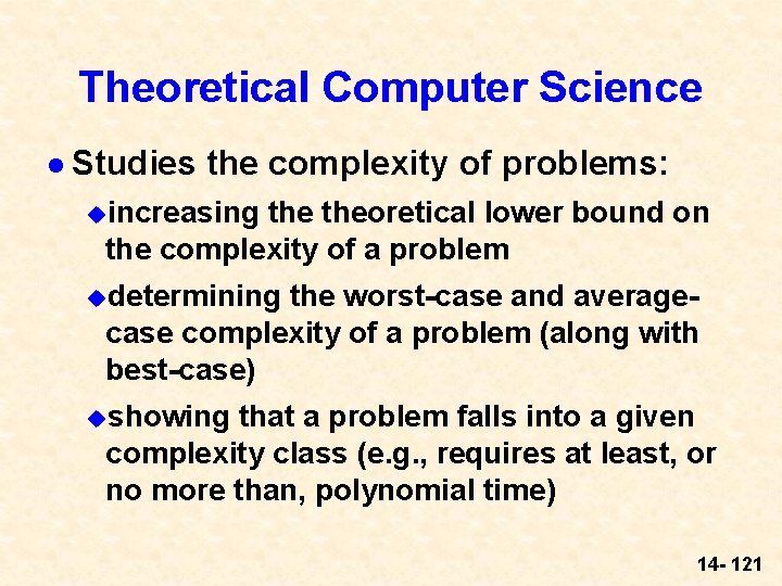
Theoretical Computer Science l Studies the complexity of problems: uincreasing theoretical lower bound on the complexity of a problem udetermining the worst-case and averagecase complexity of a problem (along with best-case) ushowing that a problem falls into a given complexity class (e. g. , requires at least, or no more than, polynomial time) 14 - 121

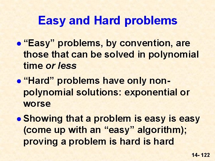
Easy and Hard problems l “Easy” problems, by convention, are those that can be solved in polynomial time or less l “Hard” problems have only nonpolynomial solutions: exponential or worse l Showing that a problem is easy (come up with an “easy” algorithm); proving a problem is hard 14 - 122

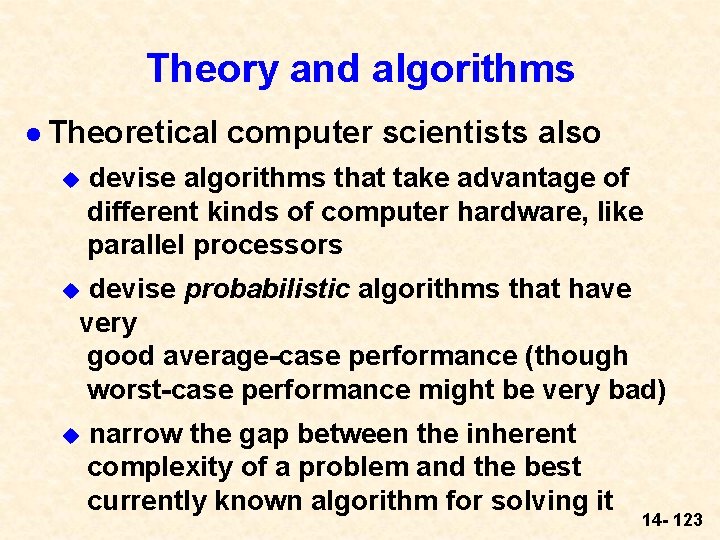
Theory and algorithms l Theoretical u computer scientists also devise algorithms that take advantage of different kinds of computer hardware, like parallel processors devise probabilistic algorithms that have very good average-case performance (though worst-case performance might be very bad) u u narrow the gap between the inherent complexity of a problem and the best currently known algorithm for solving it 14 - 123