Introduction to Computer Graphics with Web GL Ed

Introduction to Computer Graphics with Web. GL Ed Angel Professor Emeritus of Computer Science Founding Director, Arts, Research, Technology and Science Laboratory University of New Mexico Angel and Shreiner: Interactive Computer Graphics 7 E © Addison Wesley 2015 1

Homogeneous Coordinates Ed Angel Professor Emeritus of Computer Science, University of New Mexico Angel and Shreiner: Interactive Computer Graphics 7 E © Addison Wesley 2015 2

Objectives • Introduce homogeneous coordinates • Introduce change of representation for both vectors and points Angel and Shreiner: Interactive Computer Graphics 7 E © Addison Wesley 2015 3

A Single Representation If we define 0 • P = 0 and 1 • P =P then we can write v=a v +a v = [a a a 0 ] [v v v P ] T 1 1 2 2 3 3 1 2 3 0 P = P 0 + b 1 v 1+ b 2 v 2 +b 3 v 3= [b 1 b 2 b 3 1 ] [v 1 v 2 v 3 P 0] T Thus we obtain the four dimensional homogeneous coordinate representation v = [a 1 a 2 a 3 0 ] T p = [b 1 b 2 b 3 1 ] T Angel and Shreiner: Interactive Computer Graphics 7 E © Addison Wesley 2015 4

Homogeneous Coordinates and Computer Graphics • Homogeneous coordinates are key to all computer graphics systems All standard transformations (rotation, translation, scaling) can be implemented with matrix multiplications using 4 x 4 matrices Hardware pipeline works with 4 dimensional representations For orthographic viewing, we can maintain w=0 for vectors and w=1 for points For perspective we need a perspective division Angel and Shreiner: Interactive Computer Graphics 7 E © Addison Wesley 2015 5

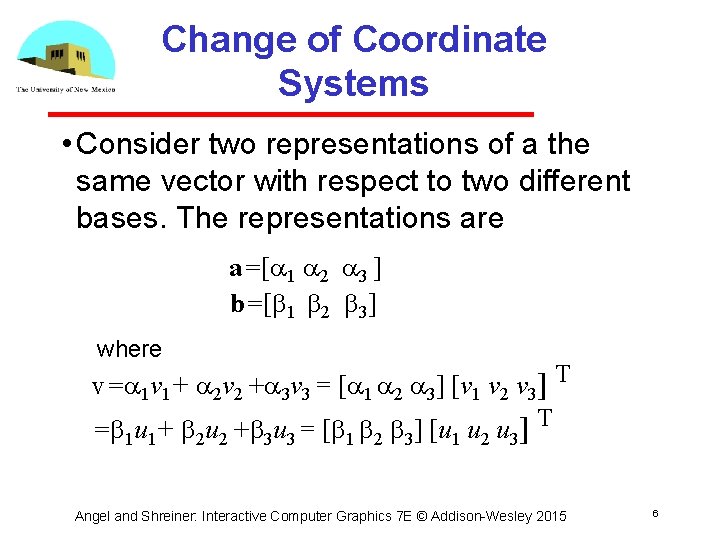
Change of Coordinate Systems • Consider two representations of a the same vector with respect to two different bases. The representations are a=[a 1 a 2 a 3 ] b=[b 1 b 2 b 3] where v=a 1 v 1+ a 2 v 2 +a 3 v 3 = [a 1 a 2 a 3] [v 1 v 2 v 3] T =b u +b u = [b b b ] [u u u ] T 1 1 2 2 3 3 1 2 3 Angel and Shreiner: Interactive Computer Graphics 7 E © Addison Wesley 2015 6

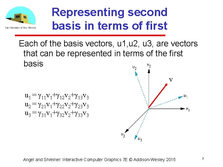
Representing second basis in terms of first Each of the basis vectors, u 1, u 2, u 3, are vectors that can be represented in terms of the first basis v u 1 = g 11 v 1+g 12 v 2+g 13 v 3 u 2 = g 21 v 1+g 22 v 2+g 23 v 3 u 3 = g 31 v 1+g 32 v 2+g 33 v 3 Angel and Shreiner: Interactive Computer Graphics 7 E © Addison Wesley 2015 7

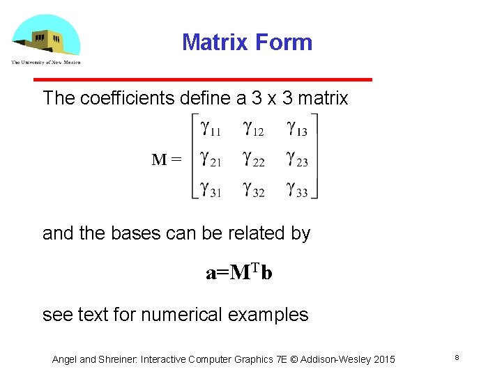
Matrix Form The coefficients define a 3 x 3 matrix M= and the bases can be related by a=MTb see text for numerical examples Angel and Shreiner: Interactive Computer Graphics 7 E © Addison Wesley 2015 8

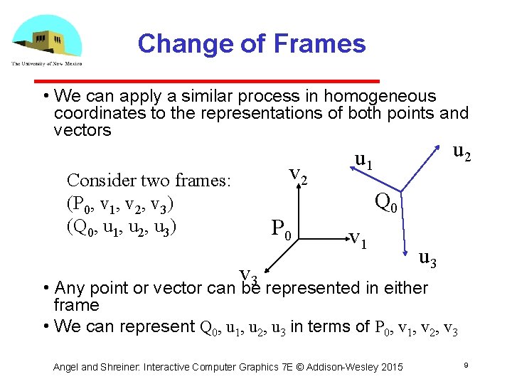
Change of Frames • We can apply a similar process in homogeneous coordinates to the representations of both points and vectors v 2 Consider two frames: (P 0, v 1, v 2, v 3) (Q 0, u 1, u 2, u 3) P 0 u 2 u 1 Q 0 v 1 v 3 u 3 • Any point or vector can be represented in either frame • We can represent Q 0, u 1, u 2, u 3 in terms of P 0, v 1, v 2, v 3 Angel and Shreiner: Interactive Computer Graphics 7 E © Addison Wesley 2015 9

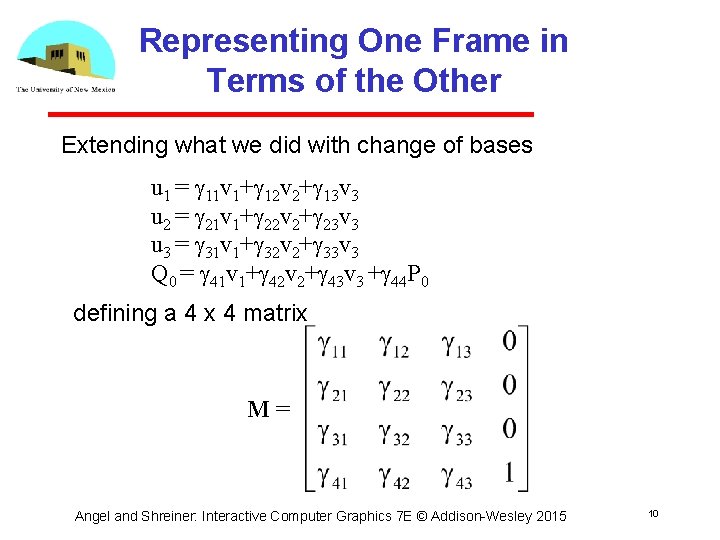
Representing One Frame in Terms of the Other Extending what we did with change of bases u 1 = g 11 v 1+g 12 v 2+g 13 v 3 u 2 = g 21 v 1+g 22 v 2+g 23 v 3 u 3 = g 31 v 1+g 32 v 2+g 33 v 3 Q 0 = g 41 v 1+g 42 v 2+g 43 v 3 +g 44 P 0 defining a 4 x 4 matrix M= Angel and Shreiner: Interactive Computer Graphics 7 E © Addison Wesley 2015 10

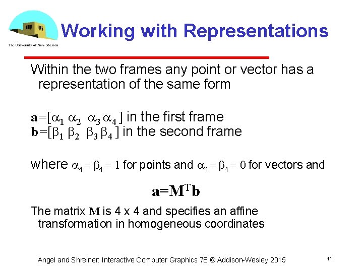
Working with Representations Within the two frames any point or vector has a representation of the same form a=[a 1 a 2 a 3 a 4 ] in the first frame b=[b 1 b 2 b 3 b 4 ] in the second frame where a 4 = b 4 = 1 for points and a 4 = b 4 = 0 for vectors and a=MTb The matrix M is 4 x 4 and specifies an affine transformation in homogeneous coordinates Angel and Shreiner: Interactive Computer Graphics 7 E © Addison Wesley 2015 11

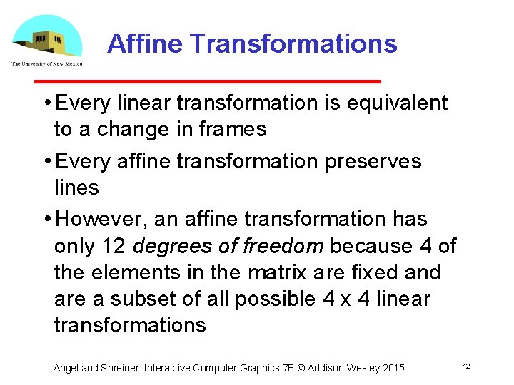
Affine Transformations • Every linear transformation is equivalent to a change in frames • Every affine transformation preserves lines • However, an affine transformation has only 12 degrees of freedom because 4 of the elements in the matrix are fixed and are a subset of all possible 4 x 4 linear transformations Angel and Shreiner: Interactive Computer Graphics 7 E © Addison Wesley 2015 12

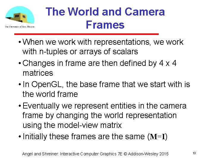
The World and Camera Frames • When we work with representations, we work with n tuples or arrays of scalars • Changes in frame are then defined by 4 x 4 matrices • In Open. GL, the base frame that we start with is the world frame • Eventually we represent entities in the camera frame by changing the world representation using the model view matrix • Initially these frames are the same (M=I) Angel and Shreiner: Interactive Computer Graphics 7 E © Addison Wesley 2015 13

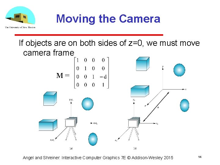
Moving the Camera If objects are on both sides of z=0, we must move camera frame M= Angel and Shreiner: Interactive Computer Graphics 7 E © Addison Wesley 2015 14