Introduction to bioinformatics Lecture 6 Pairwise sequence alignment

Introduction to bioinformatics Lecture 6 Pair-wise sequence alignment (2)

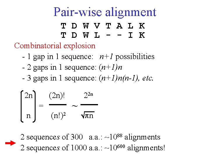
Pair-wise alignment T D W V T A L K T D W L - - I K Combinatorial explosion - 1 gap in 1 sequence: n+1 possibilities - 2 gaps in 1 sequence: (n+1)n - 3 gaps in 1 sequence: (n+1)n(n-1), etc. 2 n (2 n)! = n (n!)2 ~ 22 n n 2 sequences of 300 a. a. : ~1088 alignments 2 sequences of 1000 a. a. : ~10600 alignments!

Technique to overcome the combinatorial explosion: Dynamic Programming • Alignment is simulated as Markov process, all sequence positions are seen as independent • Chances of sequence events are independent – Therefore, probabilities per aligned position need to be multiplied – Amino acid matrices contain so-called log-odds values (log 10 of the probabilities), so probabilities can be summed

To say the same more statistically… • To perform statistical analyses on messages or sequences, we need a reference model. • The model: each letter in a sequence is selected from a defined alphabet in an independent and identically distributed (i. i. d. ) manner. • This choice of model system will allow us to compute the statistical significance of certain characteristics of a sequence, its subsequences, or an alignment. • Given a probability distribution, Pi, for the letters in a i. i. d. message, the probability of seeing a particular sequence of letters i, j, k, . . . n is simply Pi Pj Pk···Pn. • As an alternative to multiplication of the probabilities, we could sum their logarithms and exponentiate the result. The probability of the same sequence of letters can be computed by exponentiating log Pi + log Pj + log Pk+ ··· + log Pn. • In practice, when aligning sequences we only add log-odds values (residue exchange matrix) but we do not exponentiate the final score.

Sequence alignment History of Dynamic Programming algorithm 1970 Needleman-Wunsch global pair-wise alignment Needleman SB, Wunsch CD (1970) A general method applicable to the search for similarities in the amino acid sequence of two proteins, J Mol Biol. 48(3): 443 -53. 1981 Smith-Waterman local pair-wise alignment Smith, TF, Waterman, MS (1981) Identification of common molecular subsequences. J. Mol. Biol. 147, 195 -197.

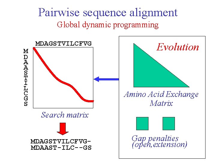
Pairwise sequence alignment Global dynamic programming M D A A S T I L C G S MDAGSTVILCFVG Evolution Amino Acid Exchange Matrix Search matrix MDAGSTVILCFVGMDAAST-ILC--GS Gap penalties (open, extension)

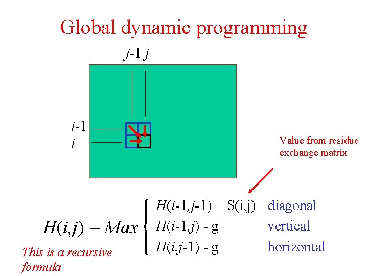
Global dynamic programming j-1 j i-1 i H(i, j) = Max This is a recursive formula Value from residue exchange matrix H(i-1, j-1) + S(i, j) diagonal H(i-1, j) - g vertical H(i, j-1) - g horizontal

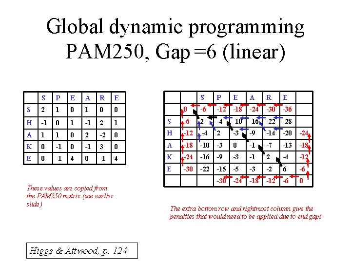
Global dynamic programming PAM 250, Gap =6 (linear) S P E A R E 0 -6 -12 -18 -24 -30 -36 S -6 2 -4 -10 -16 -22 -28 0 H -12 -4 2 -3 -9 -14 -20 -24 3 0 A -18 -10 -3 0 -1 -7 -13 -18 -1 4 K -24 -16 -9 -3 -1 2 -4 -12 E -30 -22 -15 -5 -3 -2 6 -6 -30 -24 -18 -12 -6 0 S P E A R E S 2 1 0 0 H -1 0 1 -1 2 1 A 1 1 0 2 -2 K 0 -1 E 0 -1 4 0 These values are copied from the PAM 250 matrix (see earlier slide) Higgs & Attwood, p. 124 The extra bottom row and rightmost column give the penalties that would need to be applied due to end gaps

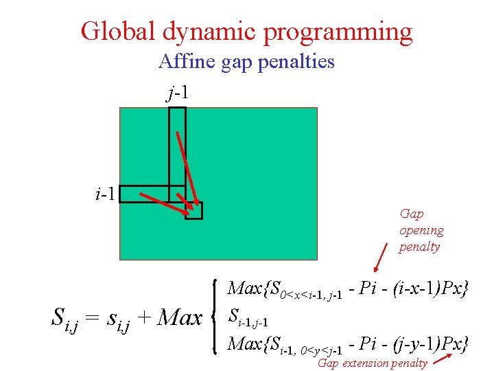
Global dynamic programming Affine gap penalties j-1 i-1 Gap opening penalty Si, j = si, j + Max{S 0<x<i-1, j-1 - Pi - (i-x-1)Px} Si-1, j-1 Max{Si-1, 0<y<j-1 - Pi - (j-y-1)Px} Gap extension penalty

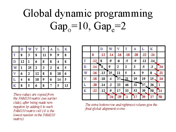
Global dynamic programming Gapo=10, Gape=2 D W V T A L K 0 -12 -14 -16 -18 -20 -22 -24 T -12 8 -9 -6 -5 -9 -11 -14 5 D -14 0 9 2 2 3 -5 -3 -34 10 6 W -16 -13 25 11 5 4 9 0 -21 6 14 5 V -18 -10 -4 37 21 19 19 15 -16 7 5 13 L -20 -14 -2 23 46 31 37 26 1 K -22 -12 -9 17 33 53 39 50 14 -34 -29 -1 17 39 27 50 D W V T A L K T 8 3 8 11 9 9 8 D 12 1 6 8 8 4 8 W 1 25 2 3 2 6 V 6 2 12 8 8 L 4 6 10 9 K 8 5 6 8 These values are copied from the PAM 250 matrix (see earlier slide), after being made nonnegative by adding 8 to each PAM 250 matrix cell (-8 is the lowest number in the PAM 250 matrix) The extra bottom row and rightmost column give the final global alignment scores

Easy DP recipe for using affine gap penalties j-1 i-1 • M[i, j] is optimal alignment (highest scoring alignment until [i, j]) • Check – preceding row until j-2: apply appropriate gap penalties – preceding row until i-2: apply appropriate gap penalties – and cell[i-1, j-1]: apply score for cell[i-1, j-1]

DP is a two-step process • Forward step: calculate scores • Trace back: start at highest score and reconstruct the path leading to the highest score – These two steps lead to the highest scoring alignment (the optimal alignment) – This is guaranteed when you use DP!

Global dynamic programming

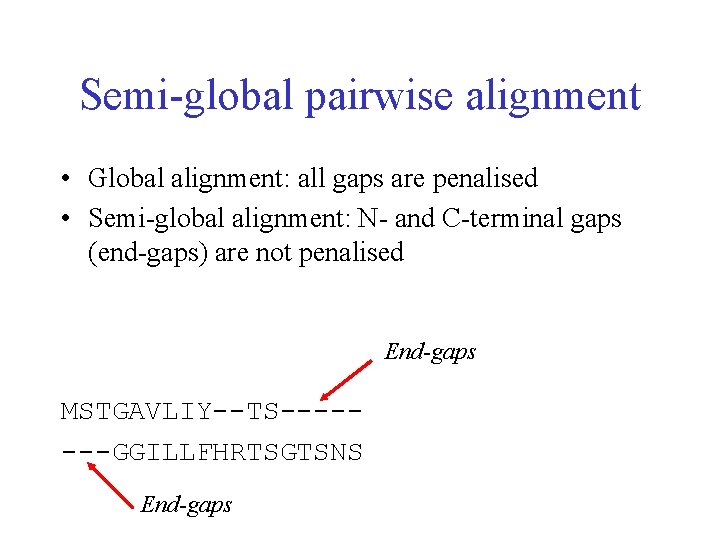
Semi-global pairwise alignment • Global alignment: all gaps are penalised • Semi-global alignment: N- and C-terminal gaps (end-gaps) are not penalised End-gaps MSTGAVLIY--TS-------GGILLFHRTSGTSNS End-gaps

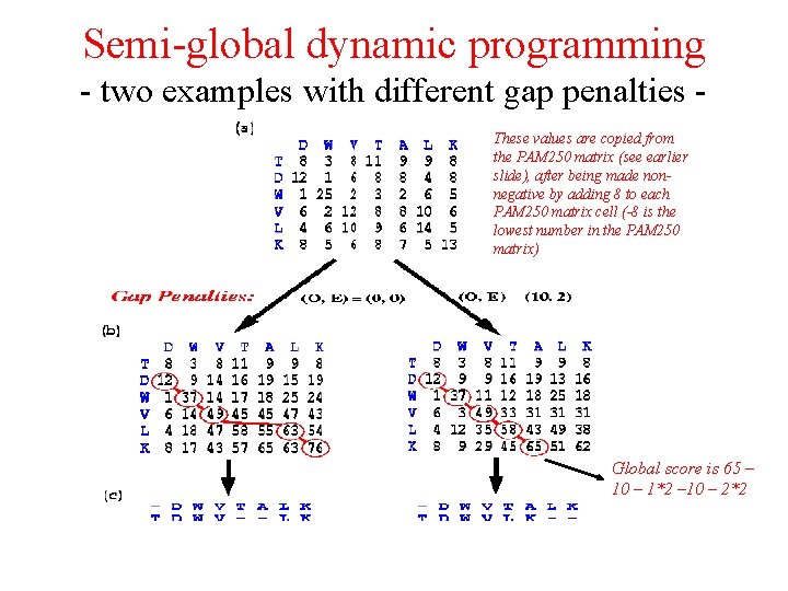
Semi-global dynamic programming - two examples with different gap penalties These values are copied from the PAM 250 matrix (see earlier slide), after being made nonnegative by adding 8 to each PAM 250 matrix cell (-8 is the lowest number in the PAM 250 matrix) Global score is 65 – 10 – 1*2 – 10 – 2*2

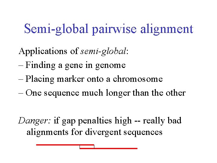
Semi-global pairwise alignment Applications of semi-global: – Finding a gene in genome – Placing marker onto a chromosome – One sequence much longer than the other Danger: if gap penalties high -- really bad alignments for divergent sequences

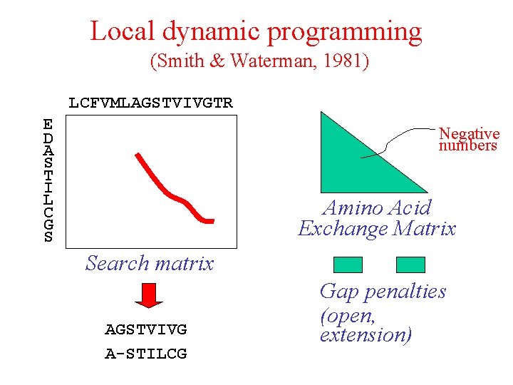
Local dynamic programming (Smith & Waterman, 1981) LCFVMLAGSTVIVGTR E D A S T I L C G S Negative numbers Amino Acid Exchange Matrix Search matrix AGSTVIVG A-STILCG Gap penalties (open, extension)

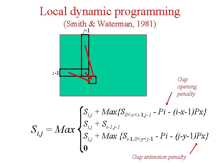
Local dynamic programming (Smith & Waterman, 1981) j-1 i-1 Si, j = Max Gap opening penalty Si, j + Max{S 0<x<i-1, j-1 - Pi - (i-x-1)Px} Si, j + Si-1, j-1 Si, j + Max {Si-1, 0<y<j-1 - Pi - (j-y-1)Px} 0 Gap extension penalty

Local dynamic programming

Dot plots • Way of representing (visualising) sequence similarity without doing dynamic programming (DP) • Make same matrix, but locally represent sequence similarity by averaging using a window

Comparing two sequences We want to be able to choose the best alignment between two sequences. A simple method of visualising similarities between two sequences is to use dot plots. The first sequence to be compared is assigned to the horizontal axis and the second is assigned to the vertical axis.

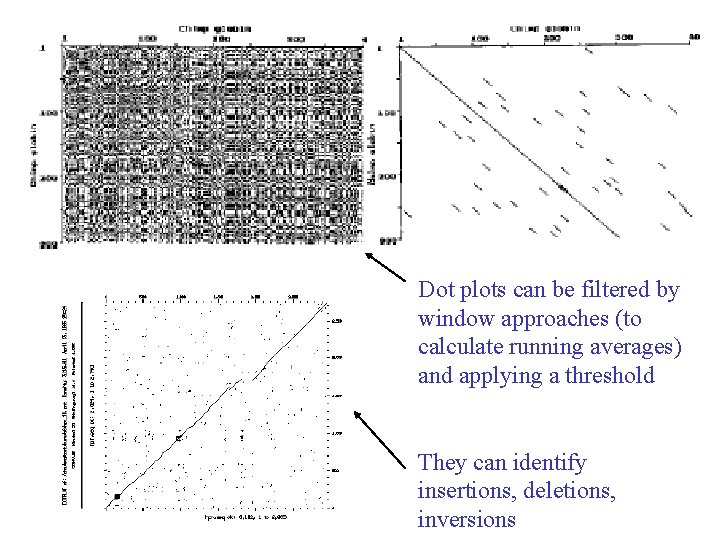
Dot plots can be filtered by window approaches (to calculate running averages) and applying a threshold They can identify insertions, deletions, inversions