Introduction to Bioinformatics 1 Introduction to Bioinformatics LECTURE

Introduction to Bioinformatics 1

Introduction to Bioinformatics. LECTURE 5: Variation within and between species * Chapter 5: Are Neanderthals among us? 2

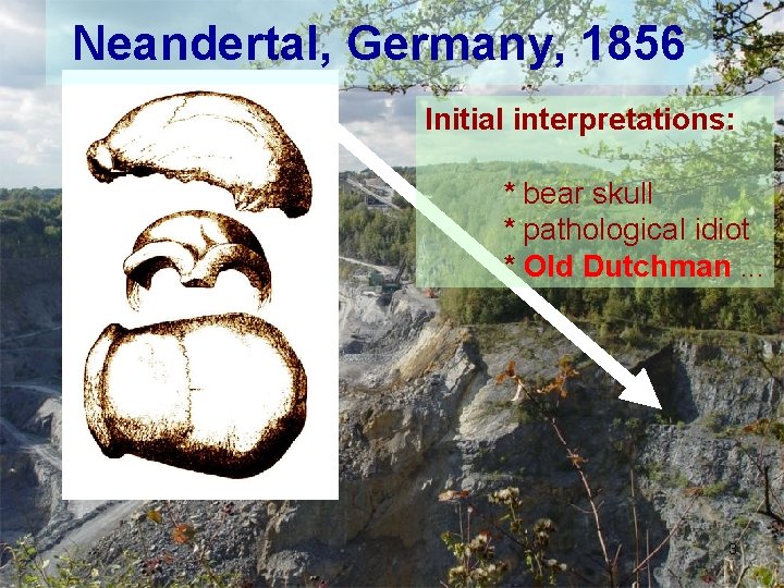
Neandertal, Germany, 1856 Initial interpretations: * bear skull * pathological idiot * Old Dutchman. . . 3

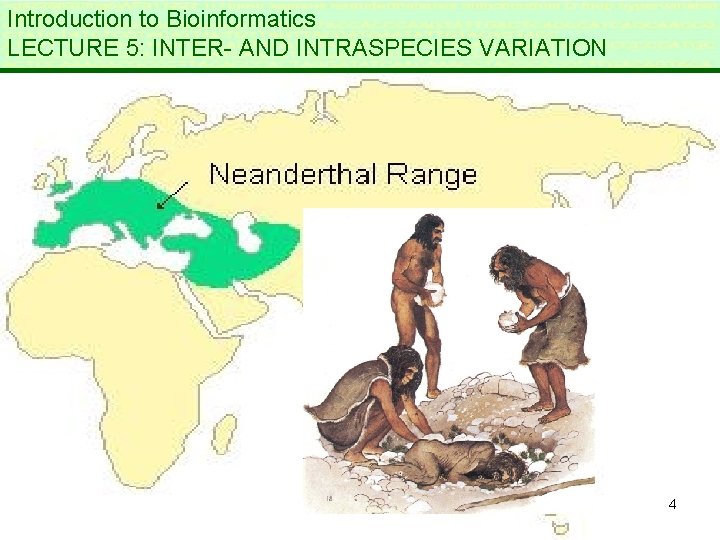
Introduction to Bioinformatics LECTURE 5: INTER- AND INTRASPECIES VARIATION 4

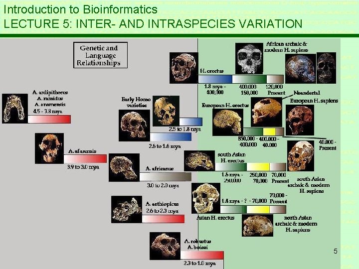
Introduction to Bioinformatics LECTURE 5: INTER- AND INTRASPECIES VARIATION 5

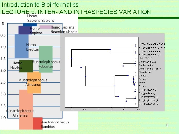
Introduction to Bioinformatics LECTURE 5: INTER- AND INTRASPECIES VARIATION 6

Introduction to Bioinformatics LECTURE 5: INTER- AND INTRASPECIES VARIATION 5. 1 Variation in DNA sequences * Even closely related individuals differ in genetic sequences * (point) mutations : copy error at certain location * Sexual reproduction – diploid genome 7

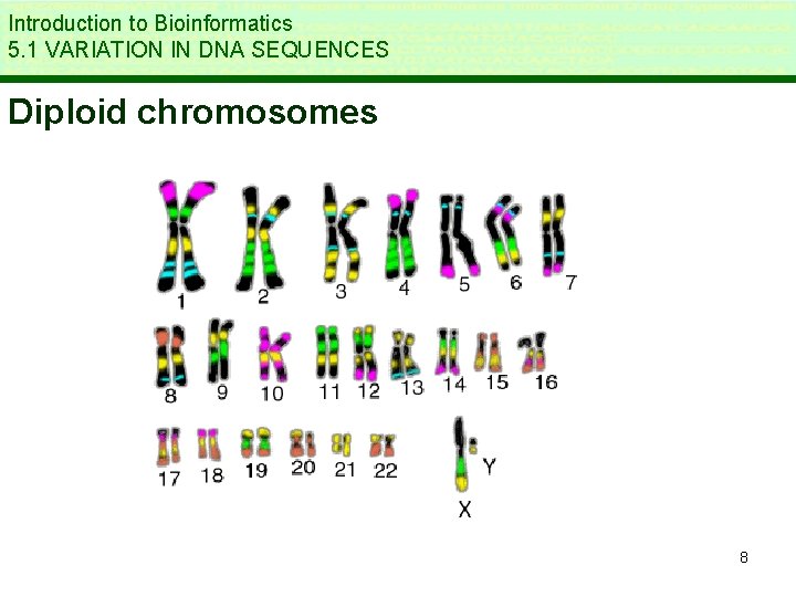
Introduction to Bioinformatics 5. 1 VARIATION IN DNA SEQUENCES Diploid chromosomes 8

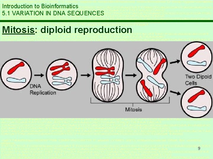
Introduction to Bioinformatics 5. 1 VARIATION IN DNA SEQUENCES Mitosis: diploid reproduction 9

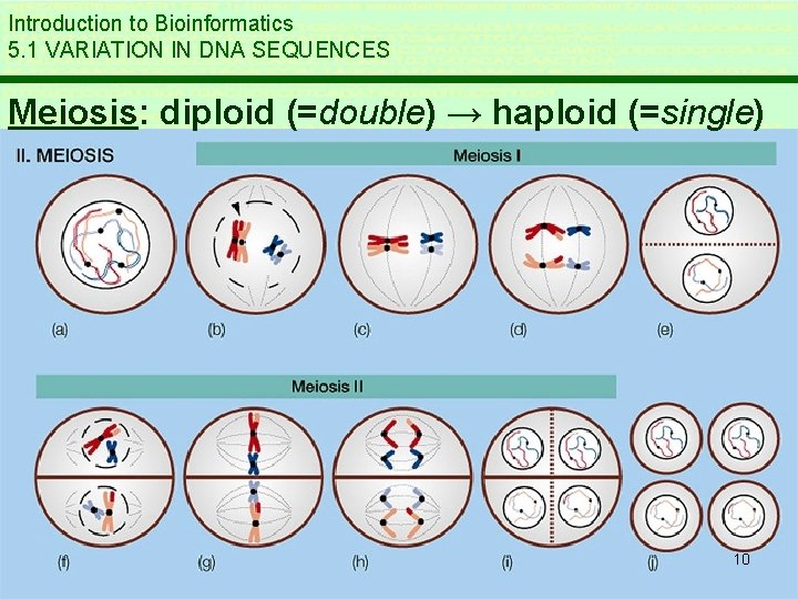
Introduction to Bioinformatics 5. 1 VARIATION IN DNA SEQUENCES Meiosis: diploid (=double) → haploid (=single) 10

Introduction to Bioinformatics 5. 1 VARIATION IN DNA SEQUENCES * typing error rate very good typist: 1 error / 1 K typed letters * all our diploid cells constantly reproduce 7 billion letters * typical cell copying error rate is ~ 1 error /1 Gbp 11

Introduction to Bioinformatics 5. 1 VARIATION IN DNA SEQUENCES GERM LINE Reverse time and follow your cells: • Now you count ~ 1013 cells • One generation ago you had 2 cells ‘somewhere’ in your parents body • Small T generations ago you had (2 T – multiple ancestors) cells • Large T generations ago you counted #(fertile ancestors) cells • Congratulations: you are 3. 4 billion years old !!! Fast-forward time and follow your cells: • Only a few cells in your reproductive organs have a chance to live on in the next generations • The rest (including you) will die … 12

Introduction to Bioinformatics 5. 1 VARIATION IN DNA SEQUENCES GERM LINE MUTATIONS This potentially immortal lineage of (germ) cells is called the GERM LINE All mutations that we have accumulated are en route on the germ line 13

Introduction to Bioinformatics 5. 1 VARIATION IN DNA SEQUENCES * Polymorphism : multiple possibilities for a nucleotide: allelle * Single Nucleotide Polymorphism – SNP (“snip”) point mutation example: AAATAAA vs AAACAAA * Humans: SNP = 1/1500 bases = 0. 067% * STR = Short Tandem Repeats (microsatelites) example: CACACACACA … * Transition - transversion 14

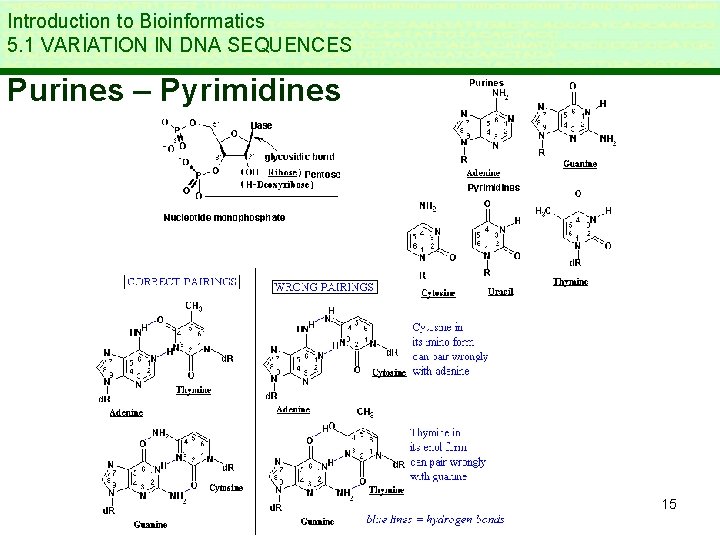
Introduction to Bioinformatics 5. 1 VARIATION IN DNA SEQUENCES Purines – Pyrimidines 15

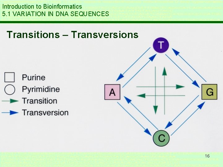
Introduction to Bioinformatics 5. 1 VARIATION IN DNA SEQUENCES Transitions – Transversions 16

Introduction to Bioinformatics LECTURE 5: INTER- AND INTRASPECIES VARIATION 5. 2 Mitochondrial DNA * mitochondriae are inherited only via the maternal line!!! * Very suitable for comparing evolution, not reshuffled 17

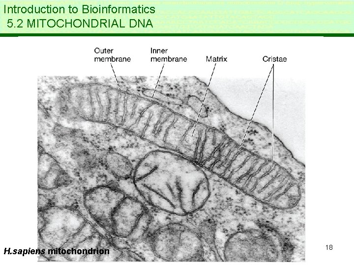
Introduction to Bioinformatics 5. 2 MITOCHONDRIAL DNA H. sapiens mitochondrion 18

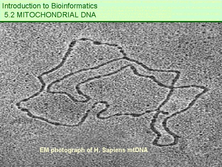
Introduction to Bioinformatics 5. 2 MITOCHONDRIAL DNA EM photograph of H. Sapiens mt. DNA 19

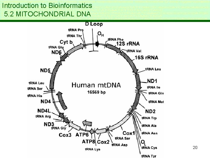
Introduction to Bioinformatics 5. 2 MITOCHONDRIAL DNA 20

Introduction to Bioinformatics LECTURE 5: INTER- AND INTRASPECIES VARIATION 5. 3 Variation between species * genetic variation accounts for morphologicalphysiological-behavioral variation * Genetic variation (c. q. distance) relates to phylogenetic relation (=relationship) * Necessity to measure distances between sequences: a metric 21

Introduction to Bioinformatics 5. 3 VARIATION BETWEEN SPECIES Substitution rate * Mutations originate in single individuals * Mutations can become fixed in a population * Mutation rate: rate at which new mutations arise * Substitution rate: rate at which a species fixes new mutations * For neutral mutations 22

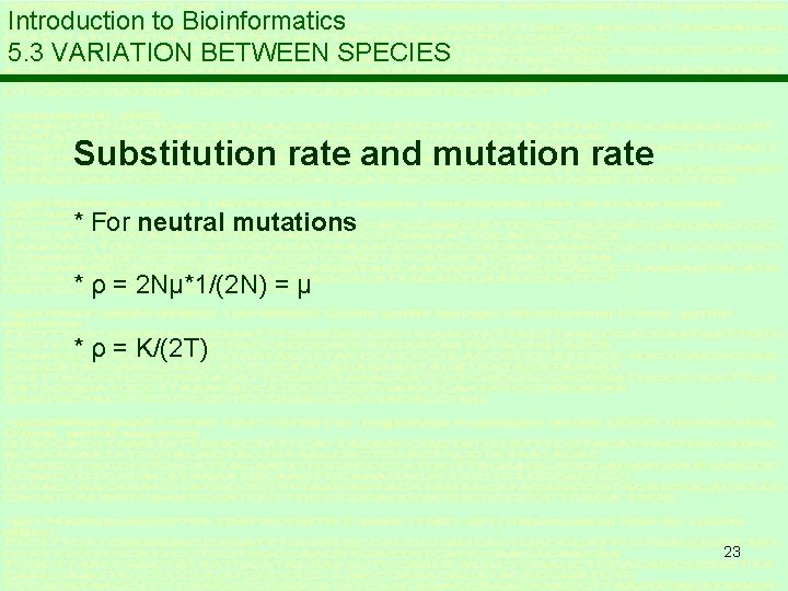
Introduction to Bioinformatics 5. 3 VARIATION BETWEEN SPECIES Substitution rate and mutation rate * For neutral mutations * ρ = 2 Nμ*1/(2 N) = μ * ρ = K/(2 T) 23

Introduction to Bioinformatics LECTURE 5: INTER- AND INTRASPECIES VARIATION 5. 4 Estimating genetic distance * Substitutions are independent (? ) * Substitutions are random * Multiple substitutions may occur * Back-mutations mutate a nucleotide back to an earlier value 24

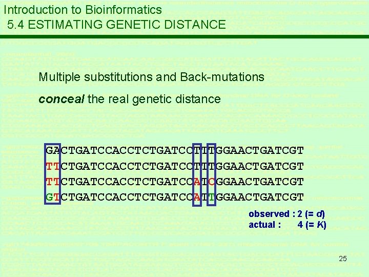
Introduction to Bioinformatics 5. 4 ESTIMATING GENETIC DISTANCE Multiple substitutions and Back-mutations conceal the real genetic distance GACTGATCCACCTCTGATCCTTTGGAACTGATCGT TTCTGATCCACCTCTGATCCATCGGAACTGATCGT GTCTGATCCACCTCTGATCCATTGGAACTGATCGT observed : 2 (= d) actual : 4 (= K) 25

Introduction to Bioinformatics 5. 4 ESTIMATING GENETIC DISTANCE * Saturation: on average one substitution per site * Two random sequences of equal length will match for approximately ¼ of their sites * In saturation therefore the proportional genetic distance is ¼ 26

Introduction to Bioinformatics 5. 4 ESTIMATING GENETIC DISTANCE * True genetic distance (proportion): K * Observed proportion of differences: d * Due to back-mutations K ≥ d 27

Introduction to Bioinformatics 5. 4 ESTIMATING GENETIC DISTANCE SEQUENCE EVOLUTION is a Markov process: a sequence at generation (= time) t depends only the sequence at generation t-1 28

Introduction to Bioinformatics 5. 4 ESTIMATING GENETIC DISTANCE The Jukes-Cantor model Correction for multiple substitutions Substitution probability per site per second is α Substitution means there are 3 possible replacements (e. g. C → {A, G, T}) Non-substitution means there is 1 possibility (e. g. C → C) 29

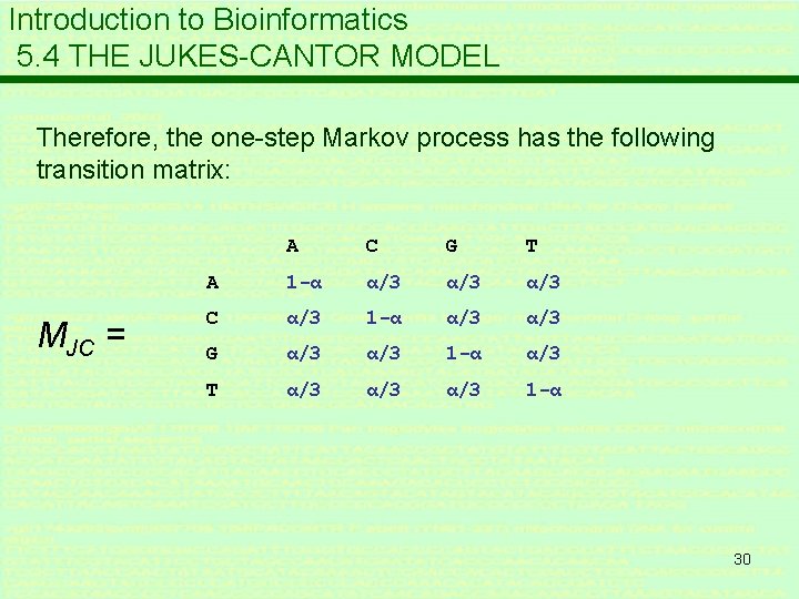
Introduction to Bioinformatics 5. 4 THE JUKES-CANTOR MODEL Therefore, the one-step Markov process has the following transition matrix: MJC = A C G T A 1 -α α/3 α/3 C α/3 1 -α α/3 G α/3 1 -α α/3 T α/3 α/3 1 -α 30

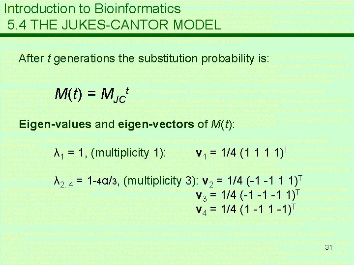
Introduction to Bioinformatics 5. 4 THE JUKES-CANTOR MODEL After t generations the substitution probability is: M(t) = MJCt Eigen-values and eigen-vectors of M(t): λ 1 = 1, (multiplicity 1): v 1 = 1/4 (1 1 1 1)T λ 2. . 4 = 1 -4α/3, (multiplicity 3): v 2 = 1/4 (-1 -1 1 1)T v 3 = 1/4 (-1 -1 -1 1)T v 4 = 1/4 (1 -1)T 31

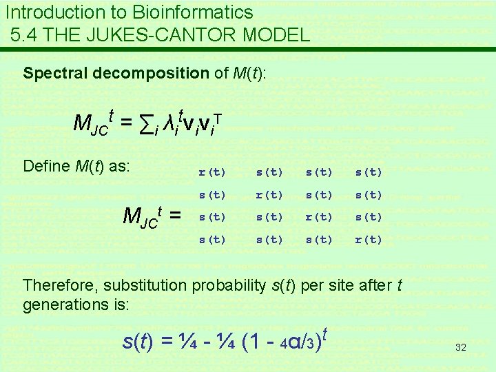
Introduction to Bioinformatics 5. 4 THE JUKES-CANTOR MODEL Spectral decomposition of M(t): MJCt = ∑i λitvivi. T Define M(t) as: MJCt = r(t) s(t) s(t) r(t) s(t) r(t) Therefore, substitution probability s(t) per site after t generations is: s(t) = ¼ - ¼ (1 - 4α/3)t 32

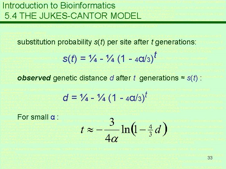
Introduction to Bioinformatics 5. 4 THE JUKES-CANTOR MODEL substitution probability s(t) per site after t generations: s(t) = ¼ - ¼ (1 - 4α/3)t observed genetic distance d after t generations ≈ s(t) : d = ¼ - ¼ (1 - 4α/3)t For small α : 33

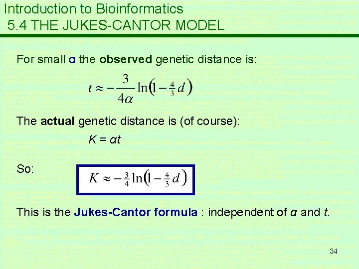
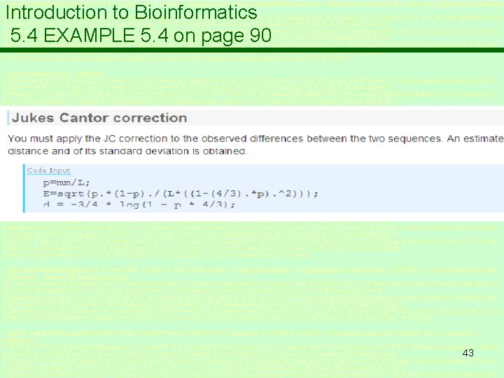
Introduction to Bioinformatics 5. 4 THE JUKES-CANTOR MODEL For small α the observed genetic distance is: The actual genetic distance is (of course): K = αt So: This is the Jukes-Cantor formula : independent of α and t. 34

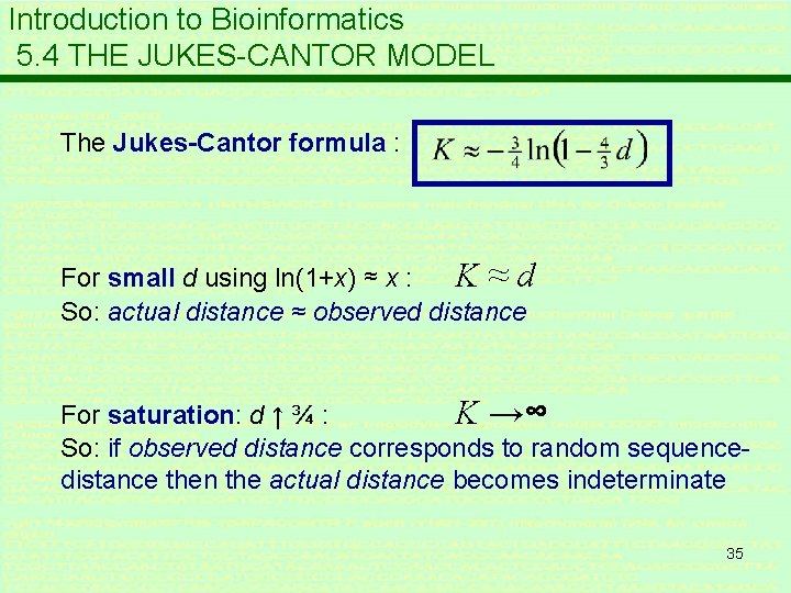
Introduction to Bioinformatics 5. 4 THE JUKES-CANTOR MODEL The Jukes-Cantor formula : For small d using ln(1+x) ≈ x : K≈d So: actual distance ≈ observed distance For saturation: d ↑ ¾ : K →∞ So: if observed distance corresponds to random sequencedistance then the actual distance becomes indeterminate 35

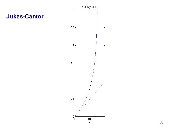
Jukes-Cantor 36

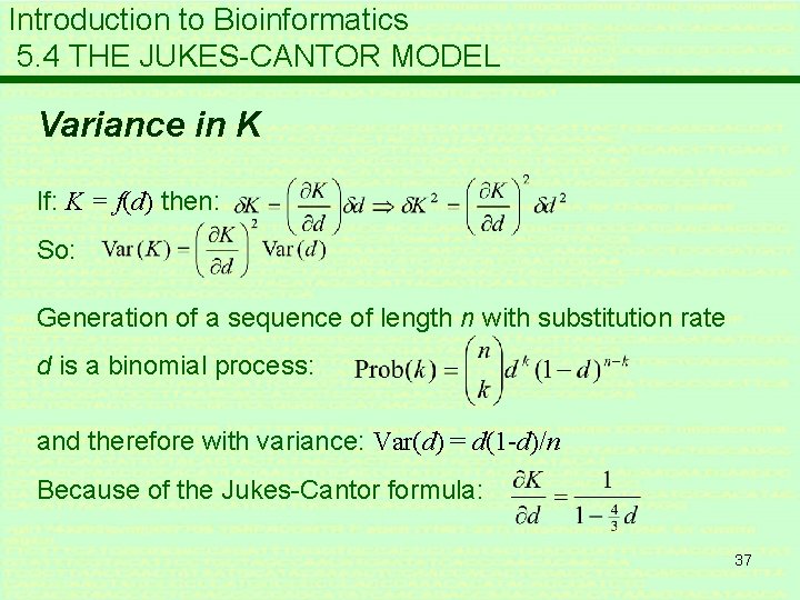
Introduction to Bioinformatics 5. 4 THE JUKES-CANTOR MODEL Variance in K If: K = f(d) then: So: Generation of a sequence of length n with substitution rate d is a binomial process: and therefore with variance: Var(d) = d(1 -d)/n Because of the Jukes-Cantor formula: 37

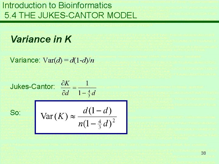
Introduction to Bioinformatics 5. 4 THE JUKES-CANTOR MODEL Variance in K Variance: Var(d) = d(1 -d)/n Jukes-Cantor: So: 38

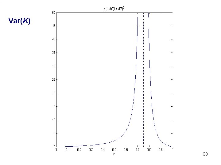
Var(K) 39

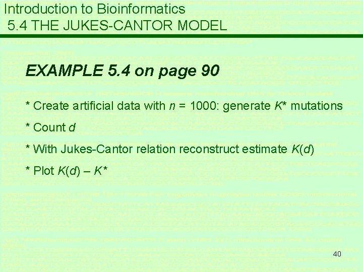
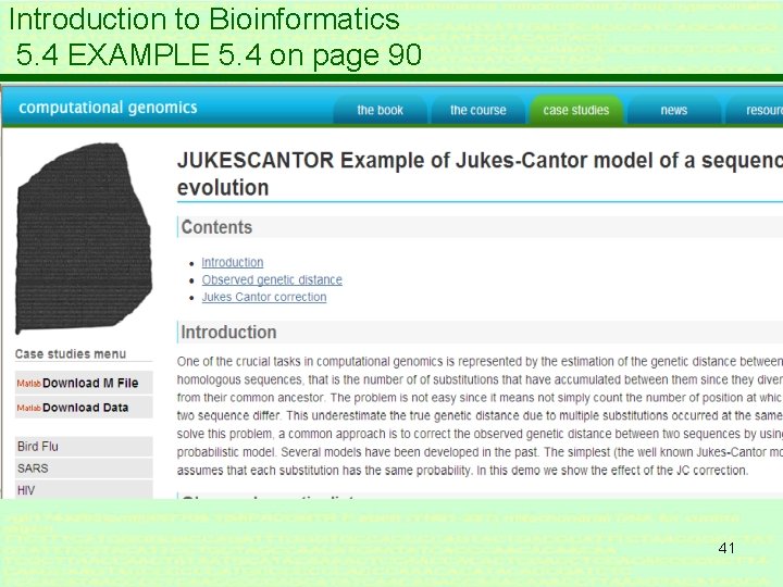
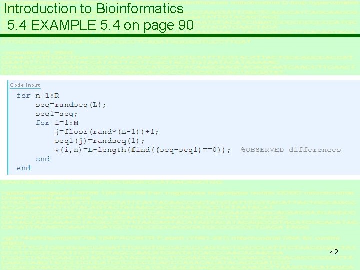
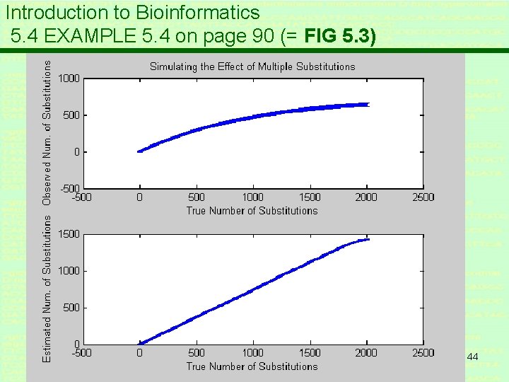
Introduction to Bioinformatics 5. 4 THE JUKES-CANTOR MODEL EXAMPLE 5. 4 on page 90 * Create artificial data with n = 1000: generate K* mutations * Count d * With Jukes-Cantor relation reconstruct estimate K(d) * Plot K(d) – K* 40

Introduction to Bioinformatics 5. 4 EXAMPLE 5. 4 on page 90 41

Introduction to Bioinformatics 5. 4 EXAMPLE 5. 4 on page 90 42

Introduction to Bioinformatics 5. 4 EXAMPLE 5. 4 on page 90 43

Introduction to Bioinformatics 5. 4 EXAMPLE 5. 4 on page 90 (= FIG 5. 3) 44

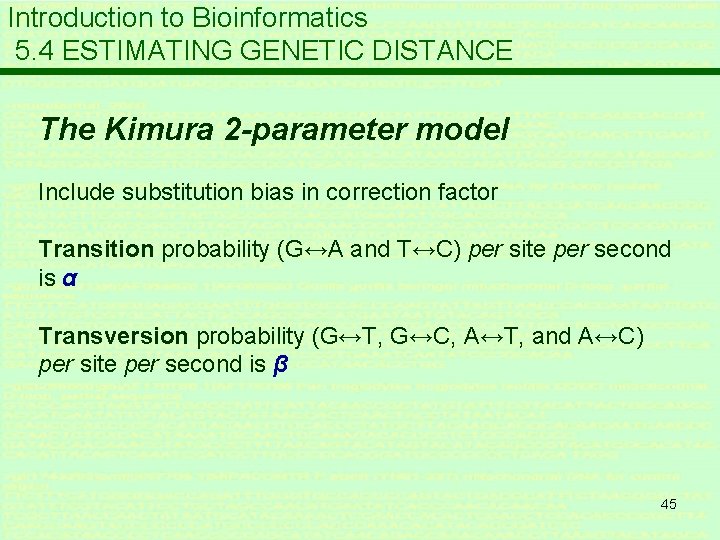
Introduction to Bioinformatics 5. 4 ESTIMATING GENETIC DISTANCE The Kimura 2 -parameter model Include substitution bias in correction factor Transition probability (G↔A and T↔C) per site per second is α Transversion probability (G↔T, G↔C, A↔T, and A↔C) per site per second is β 45

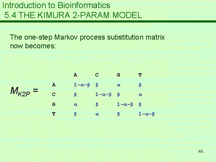
Introduction to Bioinformatics 5. 4 THE KIMURA 2 -PARAM MODEL The one-step Markov process substitution matrix now becomes: A MK 2 P = C G T A 1 -α-β β α β C β 1 -α-β β α G α β 1 -α-β β T β α β 1 -α-β 46

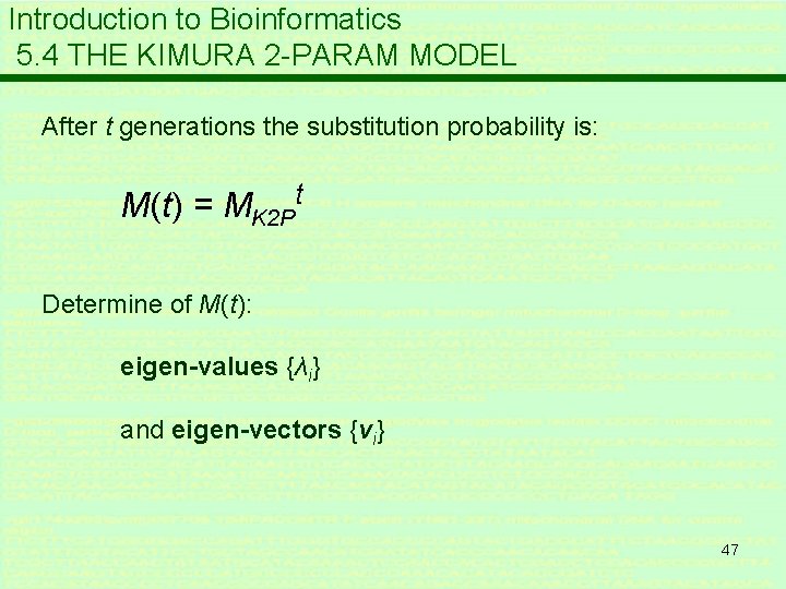
Introduction to Bioinformatics 5. 4 THE KIMURA 2 -PARAM MODEL After t generations the substitution probability is: M(t) = MK 2 Pt Determine of M(t): eigen-values {λi} and eigen-vectors {vi} 47

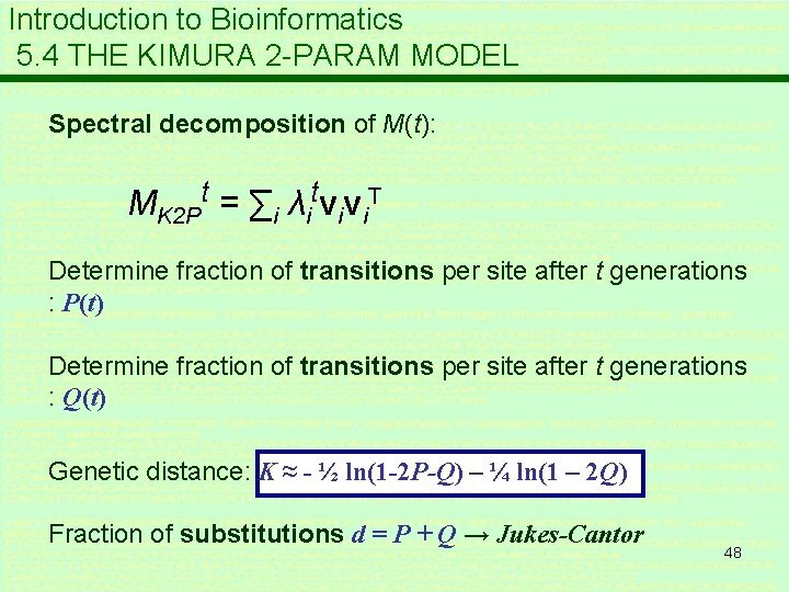
Introduction to Bioinformatics 5. 4 THE KIMURA 2 -PARAM MODEL Spectral decomposition of M(t): MK 2 Pt = ∑i λitvivi. T Determine fraction of transitions per site after t generations : P(t) Determine fraction of transitions per site after t generations : Q(t) Genetic distance: K ≈ - ½ ln(1 -2 P-Q) – ¼ ln(1 – 2 Q) Fraction of substitutions d = P + Q → Jukes-Cantor 48

Introduction to Bioinformatics 5. 4 ESTIMATING GENETIC DISTANCE Other models for nucleotide evolution * Different types of transitions/transversions * Pairwise substitutions GTR (= General Time Reversible) model * Amino-acid substitutions matrices *… 49

Introduction to Bioinformatics 5. 4 ESTIMATING GENETIC DISTANCE Other models for nucleotide evolution DEFICIT: all above models assume symmetric substitution probs; prob(A→T) = prob(T→A) Now strong evidence that this assumption is not true Challenge: incorporate this in a self-consistent model 50

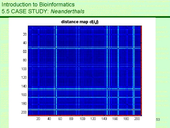
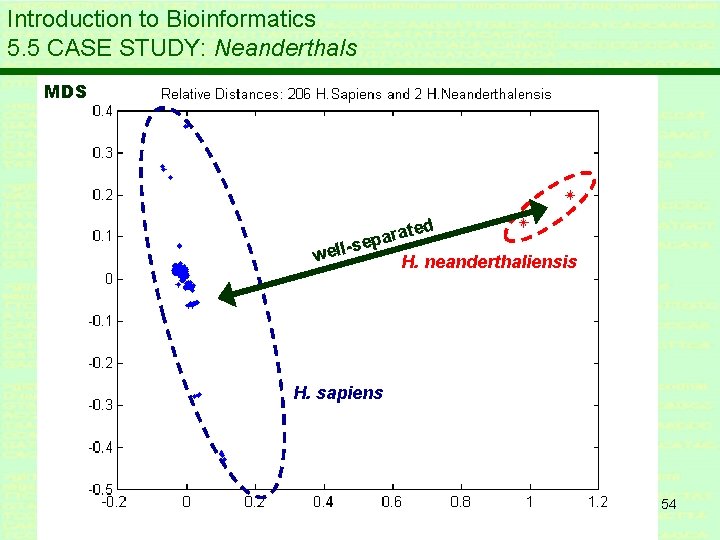
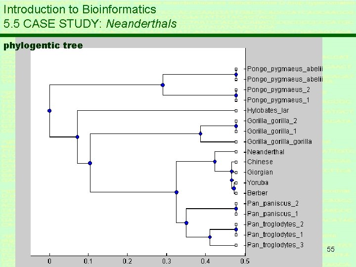
Introduction to Bioinformatics LECTURE 5: INTER- AND INTRASPECIES VARIATION 5. 5 CASE STUDY: Neanderthals * mt. DNA of 206 H. sapiens from different regions * Fragments of mt. DNA of 2 H. neanderthaliensis, including the original 1856 specimen. * all 208 samples from Gen. Bank * A homologous sequence of 800 bp of the HVR could be found in all 208 specimen. 51

Introduction to Bioinformatics 5. 5 CASE STUDY: Neanderthals * Pairwise genetic difference – corrected with Jukes-Cantor formula * d(i, j) is JC-corrected genetic difference between pair (i, j); * d. T = d * MDS (Multi Dimensional Scaling): translate distance table d to a n. D-map X, here 2 D-map 52

Introduction to Bioinformatics 5. 5 CASE STUDY: Neanderthals distance map d(i, j) 53

Introduction to Bioinformatics 5. 5 CASE STUDY: Neanderthals MDS ated r a p se well. H. neanderthaliensis H. sapiens 54

Introduction to Bioinformatics 5. 5 CASE STUDY: Neanderthals phylogentic tree 55

END of LECTURE 5 56

Introduction to Bioinformatics LECTURE 5: INTER- AND INTRASPECIES VARIATION 57

58