Introduction to asymptotic complexity Search algorithms You are

Introduction to asymptotic complexity Search algorithms You are responsible for: Weiss, chapter 5, as follows: • 5. 1 What is algorithmic analysis? • 5. 2 Examples of running time • 5. 3 NO, not responsible for this No. • 5. 4 Definition of Big-oh and Big-theta. • 5. 5 Everything except harmonic numbers. This includes the repeated doubling and repeated having stuff. • 5. 6. No, not responsible, No. Instead, you should know the following algorithms as presented in the handout on correctness of algorithms and elsewhere and be able to determine their worst-case order of execution time: linear search, finding the min, binary search, partition, insertion sort, selection sort, merge sort, quick sort. • 5. 7 Checking an algorithm analysis. • 5. 8 Limitations of big-oh analysis 0

Organization • Searching in arrays – Linear search – Binary search • Asymptotic complexity of algorithms 1

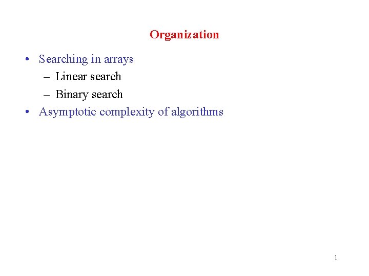
/** = index of first occ. of v in b (b. length is v not in b) */ public static boolean linear. Search(Comparable[] a, Object v) { int i = 0; // invariant: v is not in b[0. . i-1] while (i < a. length) { if (a[i]. compare. To(v) == 0) return true; i= i+1; } return false; } Linear search: 7 4 6 19 3 7 8 10 32 54 67 98 2

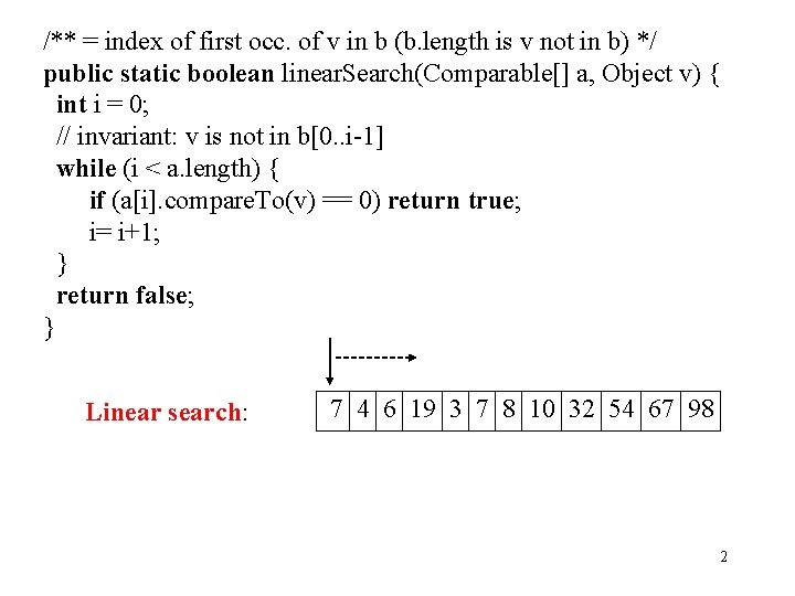
/**b is sorted. Return a value k such that b[0. . k] ≤ v < b[k+1. . ] */ public static boolean binary. Search(Comparable[] b, Object v) { int k= -1; int j= b. length; // invariant: b[0. . k] ≤ v < b[j. . ]; while (j != k+1) { int e= (k+j)/ 2; // { -1 <= k < e < j <= b. length } if (b[k]. compare. To(v) <= 0) k= e; else j= e; } Each iteration performs one return k; comparison and cuts b[k+1. . j-1] is half } 0 k e j binary search: <= v >v 3

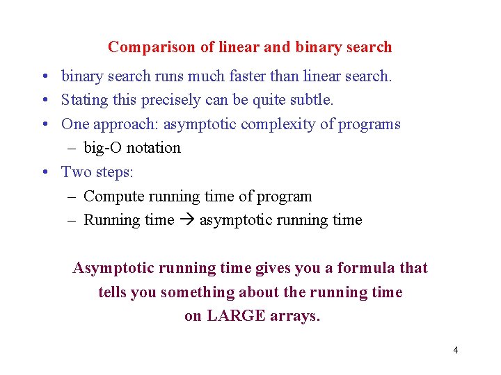
Comparison of linear and binary search • binary search runs much faster than linear search. • Stating this precisely can be quite subtle. • One approach: asymptotic complexity of programs – big-O notation • Two steps: – Compute running time of program – Running time asymptotic running time Asymptotic running time gives you a formula that tells you something about the running time on LARGE arrays. 4

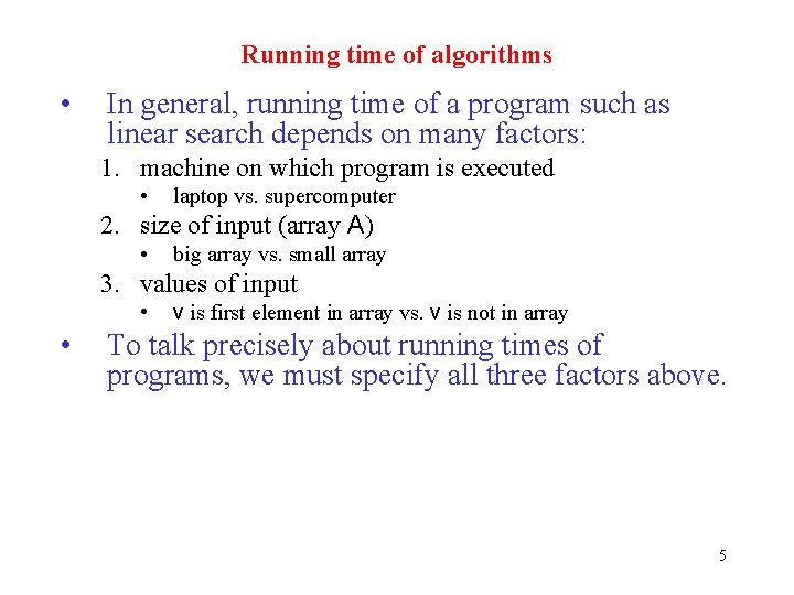
Running time of algorithms • In general, running time of a program such as linear search depends on many factors: 1. machine on which program is executed • laptop vs. supercomputer 2. size of input (array A) • big array vs. small array 3. values of input • • v is first element in array vs. v is not in array To talk precisely about running times of programs, we must specify all three factors above. 5

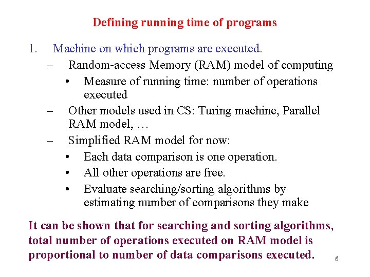
Defining running time of programs 1. Machine on which programs are executed. – Random-access Memory (RAM) model of computing • Measure of running time: number of operations executed – Other models used in CS: Turing machine, Parallel RAM model, … – Simplified RAM model for now: • Each data comparison is one operation. • All other operations are free. • Evaluate searching/sorting algorithms by estimating number of comparisons they make It can be shown that for searching and sorting algorithms, total number of operations executed on RAM model is proportional to number of data comparisons executed. 6

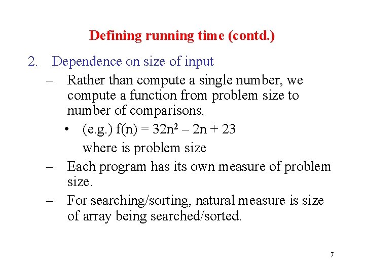
Defining running time (contd. ) 2. Dependence on size of input – Rather than compute a single number, we compute a function from problem size to number of comparisons. • (e. g. ) f(n) = 32 n 2 – 2 n + 23 where is problem size – Each program has its own measure of problem size. – For searching/sorting, natural measure is size of array being searched/sorted. 7

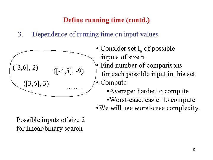
Define running time (contd. ) 3. Dependence of running time on input values ([3, 6], 2) ([3, 6], 3) ([-4, 5], -9) ……. • Consider set In of possible inputs of size n. • Find number of comparisons for each possible input in this set. • Compute • Average: harder to compute • Worst-case: easier to compute • We will use worst-case complexity. Possible inputs of size 2 for linear/binary search 8

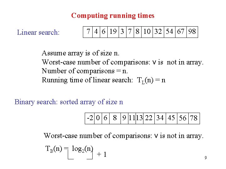
Computing running times Linear search: 7 4 6 19 3 7 8 10 32 54 67 98 Assume array is of size n. Worst-case number of comparisons: v is not in array. Number of comparisons = n. Running time of linear search: TL(n) = n Binary search: sorted array of size n -2 0 6 8 9 1113 22 34 45 56 78 Worst-case number of comparisons: v is not in array. TB(n) = log 2(n) +1 9

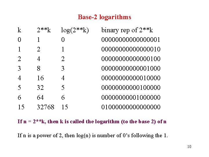
Base-2 logarithms k 0 1 2 3 4 5 6 15 2**k 1 2 4 8 16 32 64 32768 log(2**k) 0 1 2 3 4 5 6 15 binary rep of 2**k 0000000010 00000001000 000000100000 00000100000000 If n = 2**k, then k is called the logarithm (to the base 2) of n If n is a power of 2, then log(n) is number of 0’s following the 1. 10

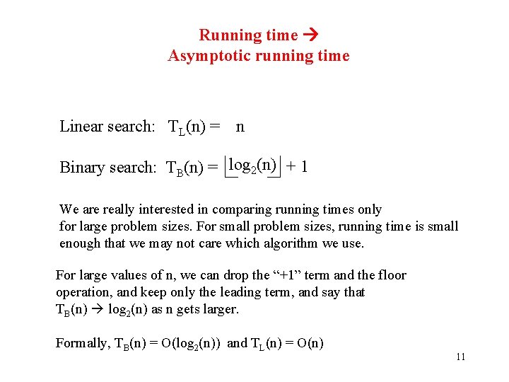
Running time Asymptotic running time Linear search: TL(n) = n Binary search: TB(n) = log 2(n) + 1 We are really interested in comparing running times only for large problem sizes. For small problem sizes, running time is small enough that we may not care which algorithm we use. For large values of n, we can drop the “+1” term and the floor operation, and keep only the leading term, and say that TB(n) log 2(n) as n gets larger. Formally, TB(n) = O(log 2(n)) and TL(n) = O(n) 11

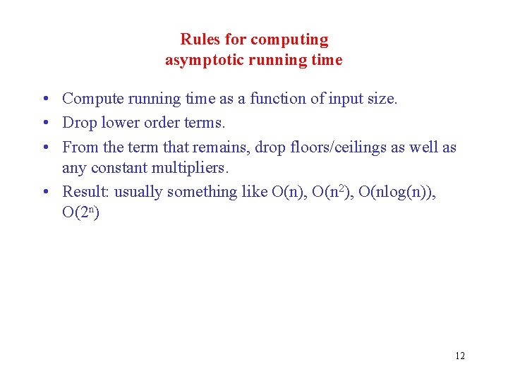
Rules for computing asymptotic running time • Compute running time as a function of input size. • Drop lower order terms. • From the term that remains, drop floors/ceilings as well as any constant multipliers. • Result: usually something like O(n), O(n 2), O(nlog(n)), O(2 n) 12

Summary of informal introduction • Asymptotic running time of a program 1. Running time: compute worst-case number of operations required to execute program on RAM model as a function of input size. – for searching/sorting algorithms, we will compute only the number of comparisons 2. Running time asymptotic running time: keep only the leading term(s) in this function. 13

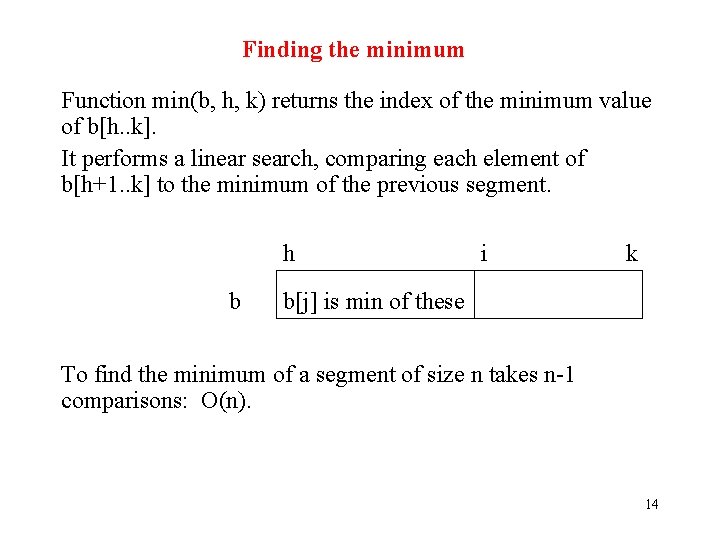
Finding the minimum Function min(b, h, k) returns the index of the minimum value of b[h. . k]. It performs a linear search, comparing each element of b[h+1. . k] to the minimum of the previous segment. h b i k b[j] is min of these To find the minimum of a segment of size n takes n-1 comparisons: O(n). 14

Selection sort: O(n**2) running time /** Sort b */ public static void selectionsort(Comparable b[]) { // inv: b[0. . k-1] sorted, b[0. . k-1] ≤ b[k. . ] k for (int k= 0; k != b. length; k= k+1) { 0 int t= min(b, k, b. length); 1 Swap b[k] and b[t]; 2 k= k+1; 3 } … } n-1 # comp. n-1 n-2 n-3 n-4 … 0 0 (n-1)*n/2 b sorted, <= k n >= = n**2 - n / 2 15