Introduction to Artificial Intelligence Unit 6 B Planning

Introduction to Artificial Intelligence – Unit 6 B Planning Course 67842 The Hebrew University of Jerusalem School of Engineering and Computer Science Instructor: Jeff Rosenschein (Chapter 10, “Artificial Intelligence: A Modern Approach”)

Outline �Planning with propositional logic (SAT) ◦ Searching in State-space �Partial-order planning ◦ Searching in Plan-space � (Planning in tirgul) Graphs, addition to material you saw 2

Planning via SAT – Motivation �Solvers have been developed for many NPcomplete classes of problems �Progress in solving SAT is probably the most prominent example �Can we do STRIPS planning via SAT? �Problem: STRIPS planning is PSPACE-complete ◦ PSPACE: “the set of all decision problems which can be solved by a Turing machine using a polynomial amount of space”; superset of NP; widely suspected to be a strict superset of NP �Solution: Bounded-STRIPS planning is in NP 3

Planning as Satisfiability � Transform the Planning problem into a series of SATs � Create a CNF that is satisfiable iff there exists a plan with b steps that satisfies the goal � Use DPLL or Walk. SAT, etc. � If successful, output the Plan that is encoded by the satisfying assignment � If not successful, b : = b + 1, continue 4

REVIEW: Efficient propositional inference Two families of efficient algorithms for propositional inference: � Complete backtracking search algorithms ◦ DPLL algorithm (Davis, Putnam, Logemann, Loveland) � Incomplete local search algorithms ◦ Walk. SAT algorithm 5

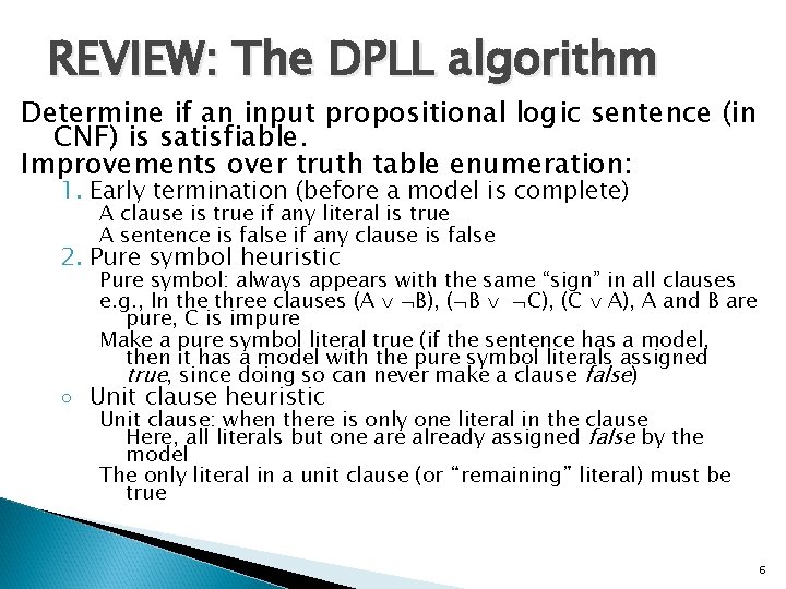
REVIEW: The DPLL algorithm Determine if an input propositional logic sentence (in CNF) is satisfiable. Improvements over truth table enumeration: 1. Early termination (before a model is complete) A clause is true if any literal is true A sentence is false if any clause is false 2. Pure symbol heuristic Pure symbol: always appears with the same “sign” in all clauses e. g. , In the three clauses (A B), ( B C), (C A), A and B are pure, C is impure Make a pure symbol literal true (if the sentence has a model, then it has a model with the pure symbol literals assigned true, since doing so can never make a clause false) ◦ Unit clause heuristic Unit clause: when there is only one literal in the clause Here, all literals but one are already assigned false by the model The only literal in a unit clause (or “remaining” literal) must be true 6

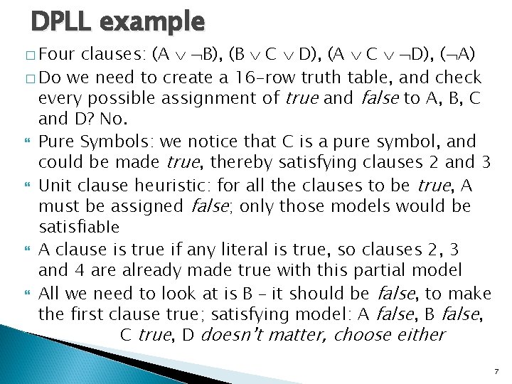
DPLL example � Four clauses: (A B), (B C D), (A C D), ( A) � Do we need to create a 16 -row truth table, and check every possible assignment of true and false to A, B, C and D? No. Pure Symbols: we notice that C is a pure symbol, and could be made true, thereby satisfying clauses 2 and 3 Unit clause heuristic: for all the clauses to be true, A must be assigned false; only those models would be satisfiable A clause is true if any literal is true, so clauses 2, 3 and 4 are already made true with this partial model All we need to look at is B – it should be false, to make the first clause true; satisfying model: A false, B false, C true, D doesn’t matter, choose either 7

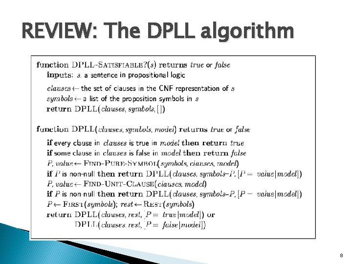
REVIEW: The DPLL algorithm 8

REVIEW: The Walk. SAT algorithm �Incomplete, local search algorithm �Evaluation function: The minconflict heuristic of minimizing the number of unsatisfied clauses (i. e. , maximizes satisfied clauses) �Balance between greediness and randomness 9

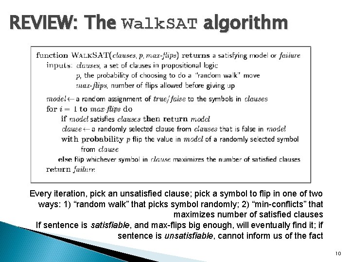
REVIEW: The Walk. SAT algorithm Every iteration, pick an unsatisfied clause; pick a symbol to flip in one of two ways: 1) “random walk” that picks symbol randomly; 2) “min-conflicts” that maximizes number of satisfied clauses If sentence is satisfiable, and max-flips big enough, will eventually find it; if sentence is unsatisfiable, cannot inform us of the fact 10

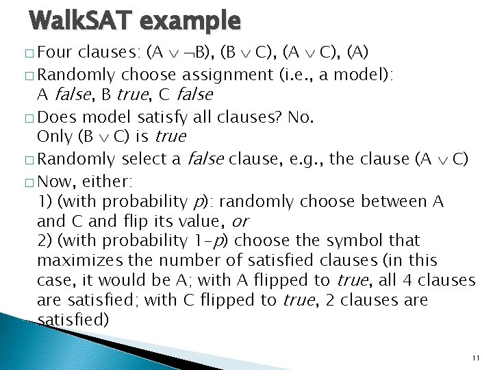
Walk. SAT example � Four clauses: (A B), (B C), (A) � Randomly choose assignment (i. e. , a model): A false, B true, C false � Does model satisfy all clauses? No. Only (B C) is true � Randomly select a false clause, e. g. , the clause (A C) � Now, either: 1) (with probability p): randomly choose between A and C and flip its value, or 2) (with probability 1 -p) choose the symbol that maximizes the number of satisfied clauses (in this case, it would be A; with A flipped to true, all 4 clauses are satisfied; with C flipped to true, 2 clauses are satisfied) 11

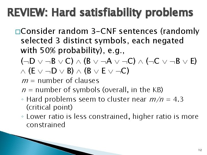
REVIEW: Hard satisfiability problems �Consider random 3 -CNF sentences (randomly selected 3 distinct symbols, each negated with 50% probability), e. g. , ( D B C) (B A C) ( C B E) (E D B) (B E C) m = number of clauses n = number of symbols (overall, in the KB) ◦ Hard problems seem to cluster near m/n = 4. 3 (critical point) ◦ Lower ratio is less constrained, higher ratio is more constrained 12

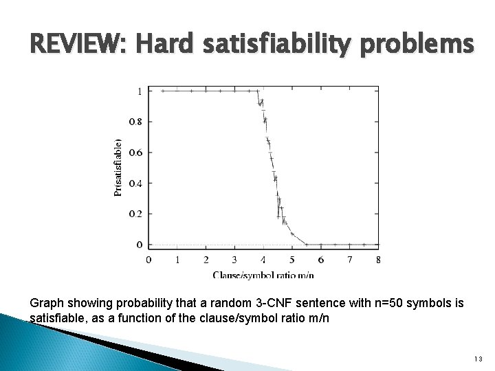
REVIEW: Hard satisfiability problems Graph showing probability that a random 3 -CNF sentence with n=50 symbols is satisfiable, as a function of the clause/symbol ratio m/n 13

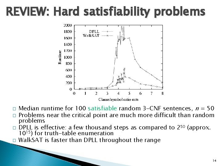
REVIEW: Hard satisfiability problems � � Median runtime for 100 satisfiable random 3 -CNF sentences, n = 50 Problems near the critical point are much more difficult than random problems DPLL is effective: a few thousand steps as compared to 250 (approx. 1015) for truth-table enumeration Walk. SAT is faster than DPLL throughout the range 14

AGAIN: Planning as Satisfiability � Transform the Planning problem into a series of SATs � Create a CNF that is satisfiable iff there exists a plan with b steps that satisfies the goal � Use DPLL or Walk. SAT, etc. � If successful, output the Plan that is encoded by the satisfying assignment � If not successful, b : = b + 1, continue 15

Questions � What notions of “steps” can we use? � What do we know about the plan we’ve found? � What should the connection be between the set of plans, and the set of satisfying assignments of the CNF encoding? � What can we say about the completeness of the algorithm? 16

STRIPS Encodings to encode b-step STRIPS plan’s existence as a CNF? � Many possible answers. Most (in use up to now) share: � How ◦ Time steps 0 <= t <= b ◦ Fact variables pt: is p TRUE or FALSE at time t ◦ Action variables at: is action a performed at time t � The size of the encoding grows linearly in b 17

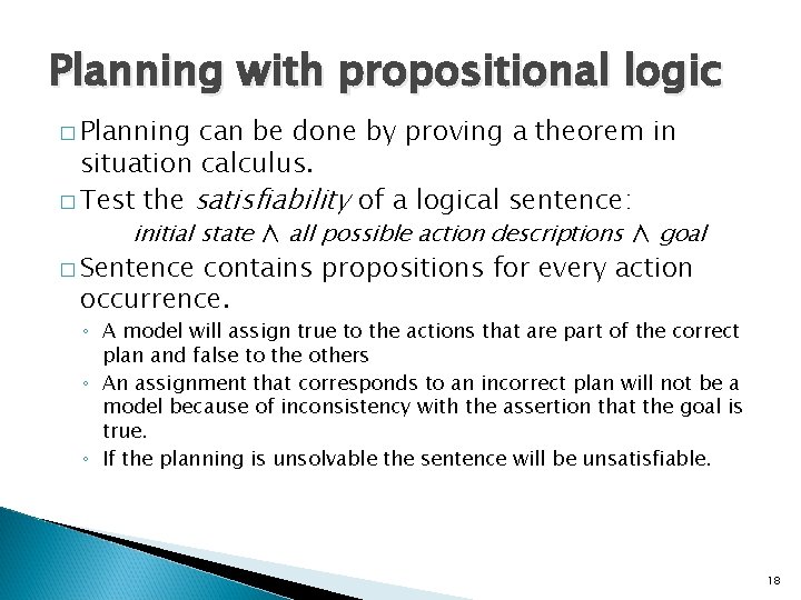
Planning with propositional logic � Planning can be done by proving a theorem in situation calculus. � Test the satisfiability of a logical sentence: initial state ∧ all possible action descriptions ∧ goal � Sentence contains propositions for every action occurrence. ◦ A model will assign true to the actions that are part of the correct plan and false to the others ◦ An assignment that corresponds to an incorrect plan will not be a model because of inconsistency with the assertion that the goal is true. ◦ If the planning is unsolvable the sentence will be unsatisfiable. 18

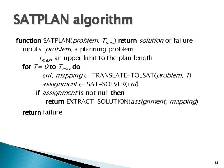
SATPLAN algorithm function SATPLAN(problem, Tmax) return solution or failure inputs: problem, a planning problem Tmax, an upper limit to the plan length for T= 0 to Tmax do cnf, mapping TRANSLATE-TO_SAT(problem, T) assignment SAT-SOLVER(cnf) if assignment is not null then return EXTRACT-SOLUTION(assignment, mapping) return failure 19

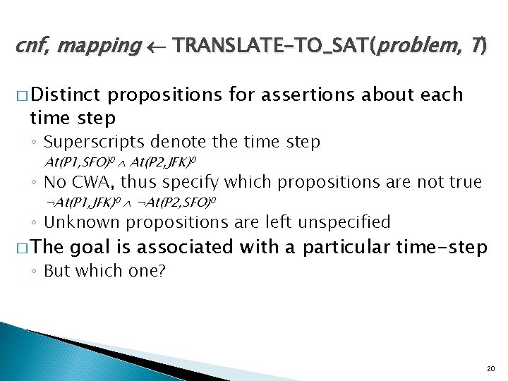
cnf, mapping TRANSLATE-TO_SAT(problem, T) � Distinct propositions for assertions about each time step ◦ Superscripts denote the time step At(P 1, SFO)0 At(P 2, JFK)0 ◦ No CWA, thus specify which propositions are not true ¬At(P 1, JFK)0 ¬At(P 2, SFO)0 ◦ Unknown propositions are left unspecified � The goal is associated with a particular time-step ◦ But which one? 20

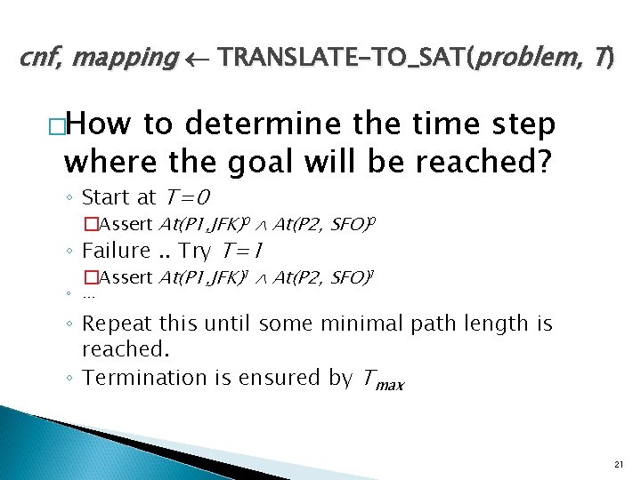
cnf, mapping TRANSLATE-TO_SAT(problem, T) �How to determine the time step where the goal will be reached? ◦ Start at T=0 �Assert At(P 1, JFK)0 At(P 2, SFO)0 ◦ Failure. . Try T=1 �Assert At(P 1, JFK)1 At(P 2, SFO)1 ◦ … ◦ Repeat this until some minimal path length is reached. ◦ Termination is ensured by Tmax 21

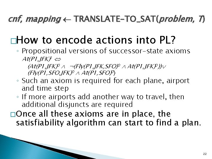
cnf, mapping TRANSLATE-TO_SAT(problem, T) �How to encode actions into PL? ◦ Propositional versions of successor-state axioms At(P 1, JFK)1 (At(P 1, JFK)0 ¬(Fly(P 1, JFK, SFO)0 At(P 1, JFK)0)) (Fly(P 1, SFO, JFK)0 At(P 1, SFO)0) ◦ Such an axiom is required for each plane, airport and time step ◦ If more airports add another way to travel, then additional disjuncts are required �Once all these axioms are in place, the satisfiability algorithm can start to find a plan. 22

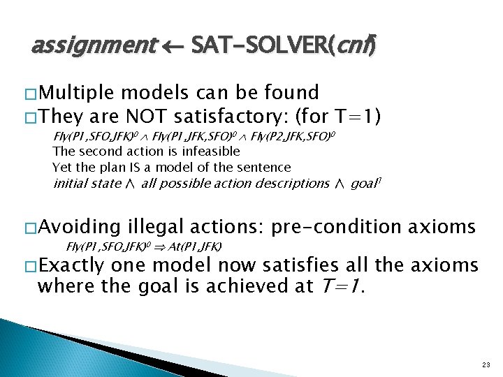
assignment SAT-SOLVER(cnf) �Multiple models can be found �They are NOT satisfactory: (for T=1) Fly(P 1, SFO, JFK)0 Fly(P 1, JFK, SFO)0 Fly(P 2, JFK, SFO)0 The second action is infeasible Yet the plan IS a model of the sentence initial state ∧ all possible action descriptions ∧ goal 1 �Avoiding illegal actions: pre-condition axioms Fly(P 1, SFO, JFK)0 At(P 1, JFK) �Exactly one model now satisfies all the axioms where the goal is achieved at T=1. 23

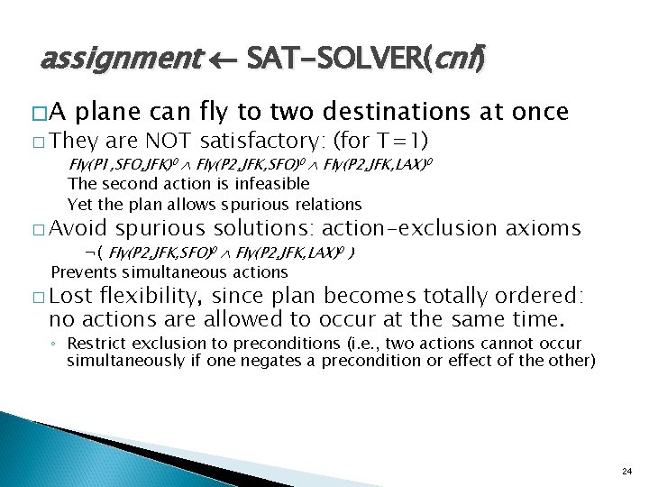
assignment SAT-SOLVER(cnf) �A plane can fly to two destinations at once � They are NOT satisfactory: (for T=1) Fly(P 1, SFO, JFK)0 Fly(P 2, JFK, SFO)0 Fly(P 2, JFK, LAX)0 The second action is infeasible Yet the plan allows spurious relations � Avoid spurious solutions: action-exclusion ¬( Fly(P 2, JFK, SFO)0 Fly(P 2, JFK, LAX)0 ) axioms Prevents simultaneous actions � Lost flexibility, since plan becomes totally ordered: no actions are allowed to occur at the same time. ◦ Restrict exclusion to preconditions (i. e. , two actions cannot occur simultaneously if one negates a precondition or effect of the other) 24

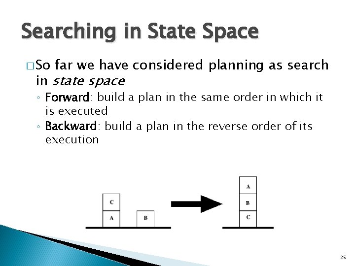
Searching in State Space � So far we have considered planning as search in state space ◦ Forward: build a plan in the same order in which it is executed ◦ Backward: build a plan in the reverse order of its execution 25

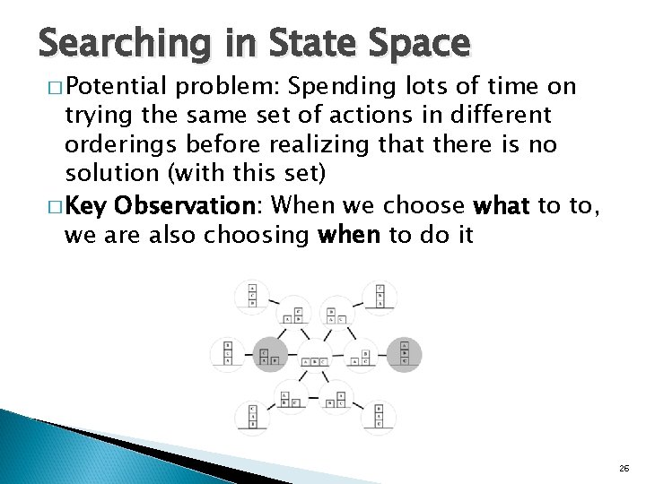
Searching in State Space � Potential problem: Spending lots of time on trying the same set of actions in different orderings before realizing that there is no solution (with this set) � Key Observation: When we choose what to to, we are also choosing when to do it 26

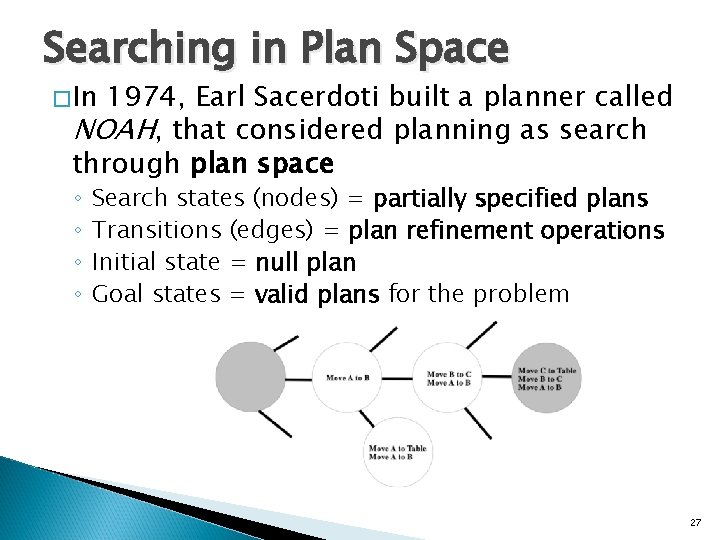
Searching in Plan Space �In 1974, Earl Sacerdoti built a planner called NOAH, that considered planning as search through plan space ◦ ◦ Search states (nodes) = partially specified plans Transitions (edges) = plan refinement operations Initial state = null plan Goal states = valid plans for the problem 27

State Space vs. Plan Space through plan space…what is a plan? �ANSWER 1: Totally ordered sequence of actions �Search ◦ But then search through state space is isomorphic to search through plan space! ◦ The nature of the space being searched is in the eye of the beholder ◦ So what’s the point of introducing “search through plan space”? �ANSWER actions 2: Partially ordered sequence of 28

Least Commitment Planning �Think how you might solve a planning problem, like… going for a vacation in Italy ◦ Need to purchase plane tickets ◦ Need to buy a “Lonely Planet” guide to Italy �BUT there is no need to decide (yet) which purchase should be done first �Least Commitment Planning ◦ Represent plans in a flexible way that enables deferring decisions ◦ At the planning phase, only the essential ordering decisions are recorded 29

Partial Order Plans �Given a STRIPS task, we search through a space of hypothetical partial order plans �A plan (= search node) is a triplet {A, O, L} in which ◦ A is a set of actions ◦ O is a set of ordering constraints ◦ L is a set of causal links �Example: �Observe: A = {a 1, a 2, a 3}, O = {a 1 < a 3, a 2 < a 3} The Planner (eventually) must do constraint satisfaction to ensure the consistency of O 30

Causal Links �A key aspect of least commitment planning is to keep track of past decisions and the reasons for those decisions ◦ If you purchase plane tickets, then make sure to bring them to the airport ◦ If another goal causes you to drop the tickets (e. g. , having you hands free to open the taxi door), then you should be sure to pick them up again ◦ A good way to reason about (and act for) non-interference between different actions introduced to the plan is to record dependencies between actions explicitly ◦ Causal links: ap ac records our decision to use ap to produce the precondition q of ac 31

Threats �Causal links are used to detect when a newly introduced action interferes with past decisions �Such an action is called a threat �Suppose that ◦ ap ac is a causal link in L (of some plan {A, O, L}), and ◦ at is yet another action in A �We say that at threatens ap ac if ◦ O union {ap < at < ac} is consistent, and ◦ q is in the delete list of at 32

Eliminating Threats � When a plan contains a threat, then it is possible that the plan will not work as anticipated � Solution: identify threats and take evasive countermeasures ◦ promotion by O union {at > ac} ◦ demotion by O union {at < ap} ◦ other possibilities… 33

Planning Problems as Null Plans � Uniformity is a key to simplicity � Can use the same structure to represent both the planning problem and complete plans � Planning problem is a null plan {A, O, L} where ◦ A = {a 0, ainf}, O = {a 0 < ainf}, L = { } ◦ pre(a 0) = { }, del(a 0) = { }, add(a 0) = I ◦ pre(ainf) = G, del(ainf) = { }, add(ainf) = { } 34

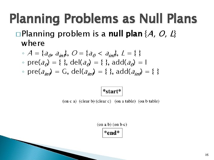
Planning Problems as Null Plans � Planning where problem is a null plan {A, O, L} ◦ A = {a 0, ainf}, O = {a 0 < ainf}, L = { } ◦ pre(a 0) = { }, del(a 0) = { }, add(a 0) = I ◦ pre(ainf) = G, del(ainf) = { }, add(ainf) = { } 35

The POP Algorithm � Algorithm that searches plan space � Starts with the null plan � Makes non-deterministic plan refinement choices until ◦ all preconditions of all actions in the plan have been supported by causal links, and ◦ all threatened causal links have been protected from possible interference 36

Shoe example Goal(Right. Shoe. On Left. Shoe. On) Init() Action(Right. Shoe, PRECOND: Right. Sock. On EFFECT: Right. Shoe. On) Action(Right. Sock, PRECOND: EFFECT: Right. Sock. On) Action(Left. Shoe, PRECOND: Left. Sock. On EFFECT: Left. Shoe. On) Action(Left. Sock, PRECOND: EFFECT: Left. Sock. On) Planner: combine two action sequences (1)leftsock, leftshoe (2)rightsock, rightshoe 37

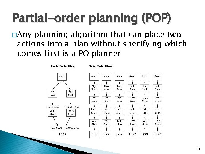
Partial-order planning (POP) �Any planning algorithm that can place two actions into a plan without specifying which comes first is a PO planner 38

POP as a search problem � States are (mostly unfinished) plans. ◦ The empty plan contains only start and finish actions � Note (again) that we are searching through the space of plans, not the space of world states 39

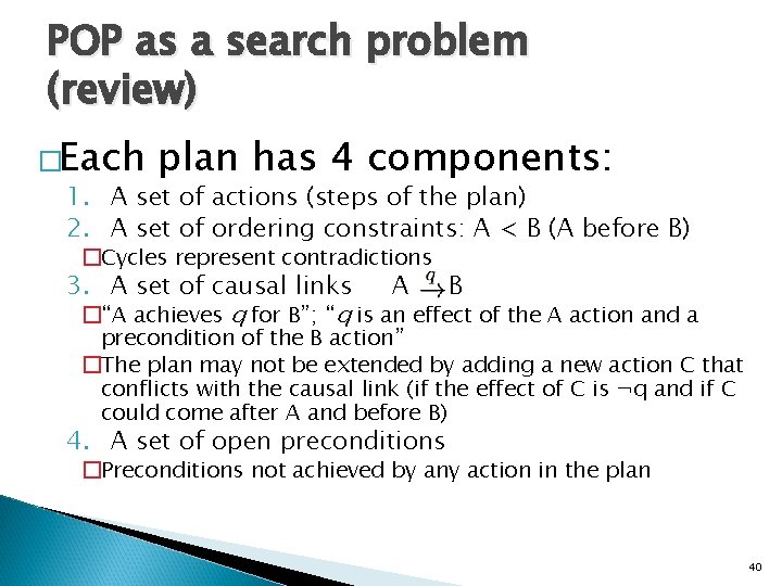
POP as a search problem (review) �Each plan has 4 components: 1. A set of actions (steps of the plan) 2. A set of ordering constraints: A < B (A before B) �Cycles represent contradictions 3. A set of causal links A B �“A achieves q for B”; “q is an effect of the A action and a precondition of the B action” �The plan may not be extended by adding a new action C that conflicts with the causal link (if the effect of C is ¬q and if C could come after A and before B) 4. A set of open preconditions �Preconditions not achieved by any action in the plan 40

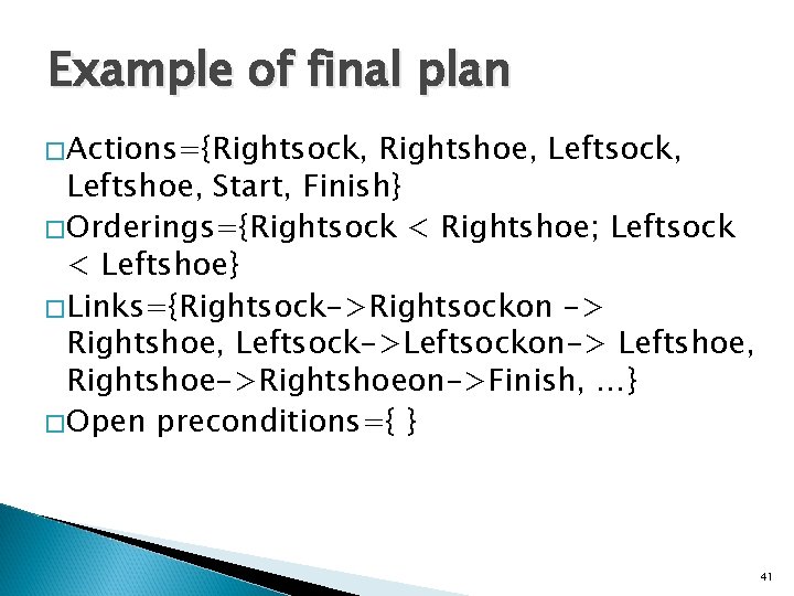
Example of final plan �Actions={Rightsock, Rightshoe, Leftsock, Leftshoe, Start, Finish} �Orderings={Rightsock < Rightshoe; Leftsock < Leftshoe} �Links={Rightsock->Rightsockon -> Rightshoe, Leftsock->Leftsockon-> Leftshoe, Rightshoe->Rightshoeon->Finish, …} �Open preconditions={ } 41

POP as a search problem plan is consistent iff there are no cycles in the ordering constraints and no conflicts with the causal links �A consistent plan with no open preconditions is a solution �A partial order plan is executed by repeatedly choosing any of the possible next actions �A 42

Solving POP �Assume propositional planning problems: ◦ The initial plan contains Start and Finish, the ordering constraint Start < Finish, no causal links, all the preconditions in Finish are open. ◦ Successor function : �picks one open precondition p on an action B and �generates a successor plan for every possible consistent way of choosing action A that achieves p. ◦ Test goal 43

Enforcing consistency �When generating successor plan: ◦ The causal link A->p->B and the ordering constraint A < B is added to the plan. �If A is new, also add start < A and A < B and A < finish to the plan ◦ Resolve conflicts between new causal link and all existing actions, e. g. , C (put in ordering constraints that make C occur outside “protection interval”) ◦ Resolve conflicts between action A (if new) and all existing causal links 44

Process summary � Operators on partial plans ◦ Add link from existing plan to open precondition ◦ Add a step to fulfill an open precondition ◦ Order one step w. r. t. another to remove possible conflicts � Gradually move from incomplete/vague plans to complete/correct plans � Backtrack if an open condition is unachievable or if a conflict is irresolvable 45

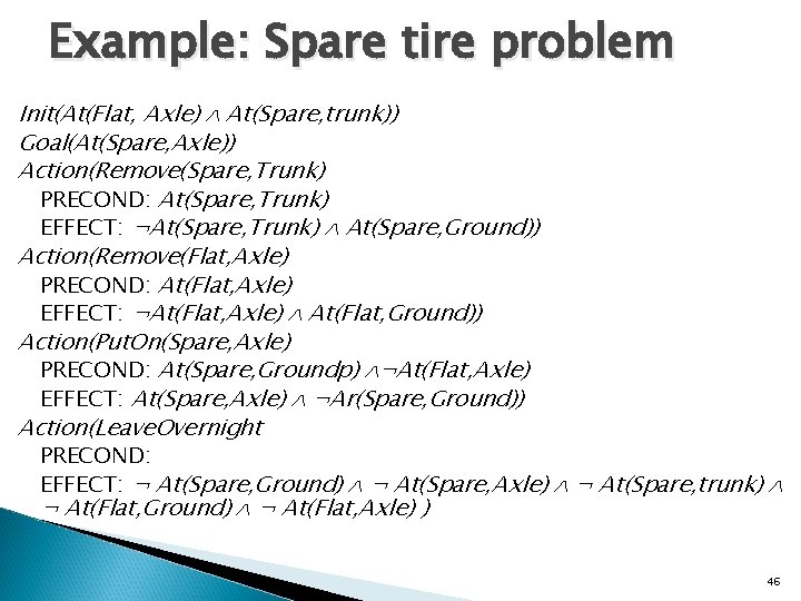
Example: Spare tire problem Init(At(Flat, Axle) At(Spare, trunk)) Goal(At(Spare, Axle)) Action(Remove(Spare, Trunk) PRECOND: At(Spare, Trunk) EFFECT: ¬At(Spare, Trunk) At(Spare, Ground)) Action(Remove(Flat, Axle) PRECOND: At(Flat, Axle) EFFECT: ¬At(Flat, Axle) At(Flat, Ground)) Action(Put. On(Spare, Axle) PRECOND: At(Spare, Groundp) ¬At(Flat, Axle) EFFECT: At(Spare, Axle) ¬Ar(Spare, Ground)) Action(Leave. Overnight PRECOND: EFFECT: ¬ At(Spare, Ground) ¬ At(Spare, Axle) ¬ At(Spare, trunk) ¬ At(Flat, Ground) ¬ At(Flat, Axle) ) 46

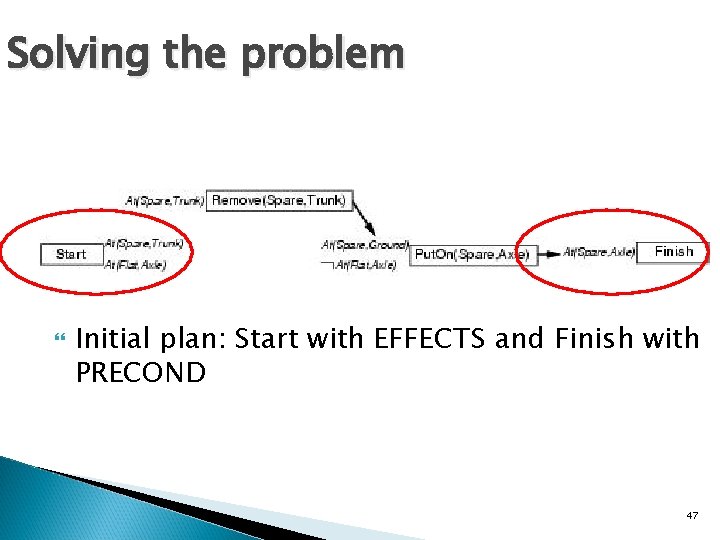
Solving the problem Initial plan: Start with EFFECTS and Finish with PRECOND 47

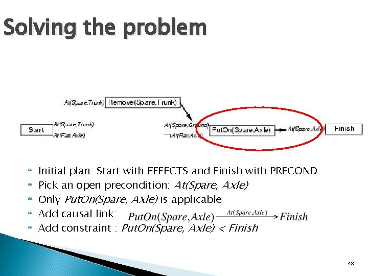
Solving the problem Initial plan: Start with EFFECTS and Finish with PRECOND Pick an open precondition: At(Spare, Axle) Only Put. On(Spare, Axle) is applicable Add causal link: Add constraint : Put. On(Spare, Axle) < Finish 48

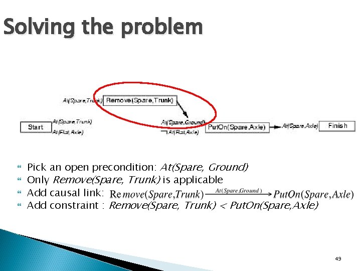
Solving the problem Pick an open precondition: At(Spare, Ground) Only Remove(Spare, Trunk) is applicable Add causal link: Add constraint : Remove(Spare, Trunk) < Put. On(Spare, Axle) 49

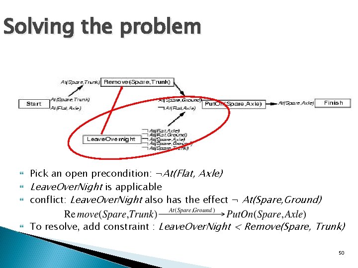
Solving the problem Pick an open precondition: ¬At(Flat, Axle) Leave. Over. Night is applicable conflict: Leave. Over. Night also has the effect ¬ At(Spare, Ground) To resolve, add constraint : Leave. Over. Night < Remove(Spare, Trunk) 50

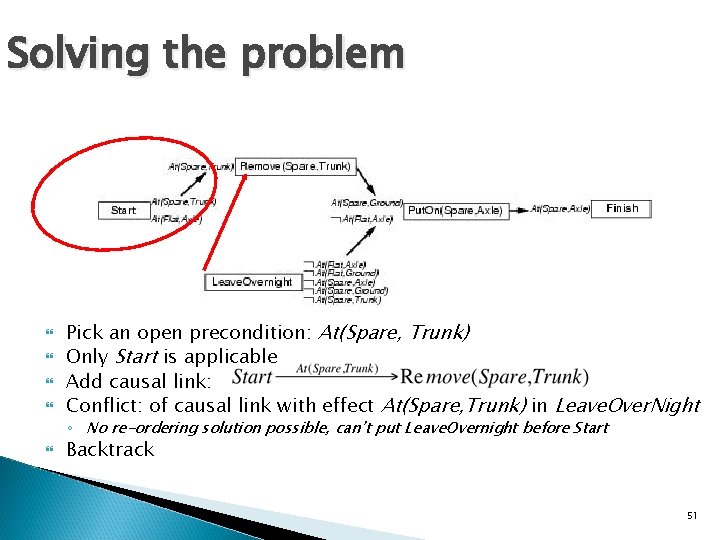
Solving the problem Pick an open precondition: At(Spare, Trunk) Only Start is applicable Add causal link: Conflict: of causal link with effect At(Spare, Trunk) in Leave. Over. Night ◦ No re-ordering solution possible, can’t put Leave. Overnight before Start Backtrack 51

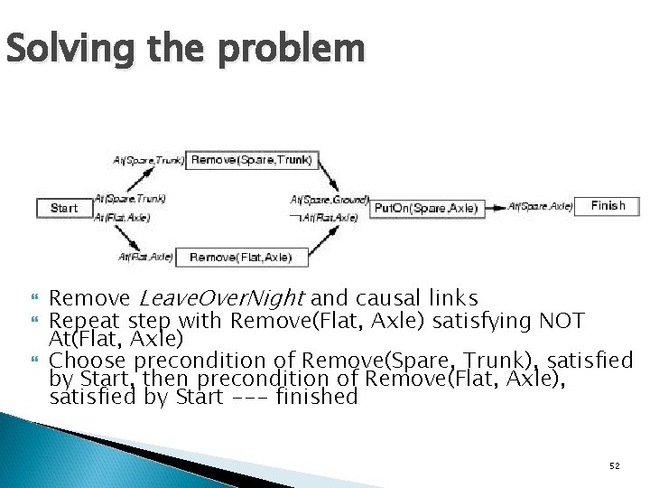
Solving the problem Remove Leave. Over. Night and causal links Repeat step with Remove(Flat, Axle) satisfying NOT At(Flat, Axle) Choose precondition of Remove(Spare, Trunk), satisfied by Start, then precondition of Remove(Flat, Axle), satisfied by Start --- finished 52

Some details … � What happens when a first-order representation that includes variables is used? ◦ Complicates the process of detecting and resolving conflicts ◦ Can be resolved by introducing inequality constraints (“there will only be a conflict if z = B”) � CSP’s most-constrained-variable constraint can be used for planning algorithms to select a PRECOND (select the open precondition that can be satisfied in the fewest number of ways) 53

Planning graphs � Used to achieve better heuristic estimates ◦ A solution can also be directly extracted using GRAPHPLAN � Consists of a sequence of levels that correspond to time steps in the plan ◦ Level 0 is the initial state ◦ Each level consists of a set of literals and a set of actions �Literals = all those that could be true at that time step, depending upon the actions executed at the preceding time step �Actions = all those actions that could have their preconditions satisfied at that time step, depending on which of the literals actually hold 54

Planning graphs � “Could”? ◦ Records only a restricted subset of possible negative interactions among actions � They work only for propositional problems � Example: Init(Have(Cake)) Goal(Have(Cake) Eaten(Cake)) Action(Eat(Cake), PRECOND: Have(Cake) EFFECT: ¬Have(Cake) Eaten(Cake)) Action(Bake(Cake), PRECOND: ¬ Have(Cake) EFFECT: Have(Cake)) 55

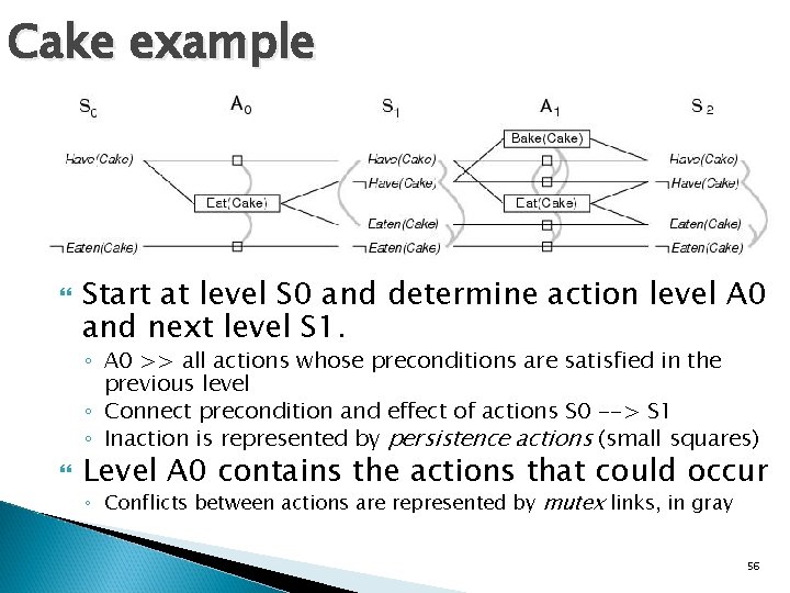
Cake example Start at level S 0 and determine action level A 0 and next level S 1. ◦ A 0 >> all actions whose preconditions are satisfied in the previous level ◦ Connect precondition and effect of actions S 0 --> S 1 ◦ Inaction is represented by persistence actions (small squares) Level A 0 contains the actions that could occur ◦ Conflicts between actions are represented by mutex links, in gray 56

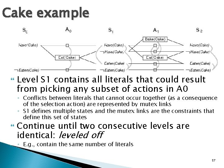
Cake example Level S 1 contains all literals that could result from picking any subset of actions in A 0 ◦ Conflicts between literals that cannot occur together (as a consequence of the selection action) are represented by mutex links ◦ S 1 defines multiple states and the mutex links are the constraints that define this set of states Continue until two consecutive levels are identical: leveled off ◦ E. g. , contain the same number of literals 57

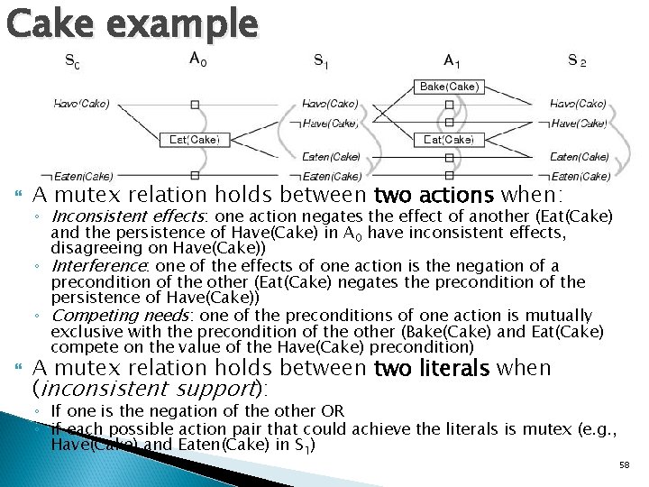
Cake example A mutex relation holds between two actions when: ◦ Inconsistent effects: one action negates the effect of another (Eat(Cake) and the persistence of Have(Cake) in A 0 have inconsistent effects, disagreeing on Have(Cake)) ◦ Interference: one of the effects of one action is the negation of a precondition of the other (Eat(Cake) negates the precondition of the persistence of Have(Cake)) ◦ Competing needs: one of the preconditions of one action is mutually exclusive with the precondition of the other (Bake(Cake) and Eat(Cake) compete on the value of the Have(Cake) precondition) A mutex relation holds between two literals when (inconsistent support): ◦ If one is the negation of the other OR ◦ if each possible action pair that could achieve the literals is mutex (e. g. , Have(Cake) and Eaten(Cake) in S 1) 58

PG and heuristic estimation � PG’s provide information about the problem ◦ A literal that does not appear in the final level of the graph cannot be achieved by any plan �Useful for backward search (cost = infinity) ◦ Level of appearance can be used as cost estimate of achieving any goal literals = level cost ◦ Small problem: several actions can occur at one level, but heuristic counts levels, not actions �Restrict to one action at any given time step using serial PG (add mutex links between every pair of actions, except persistence actions) 59

PG and heuristic estimation � Cost of a conjunction of goals? ◦ Max-level (admissable, but inaccurate), ◦ level-sum (inadmissable but works well in practice), and ◦ set-level (the level at which all conjuncts appear without any pair being mutually exclusive) heuristics PG is a relaxed problem (if a literal does not appear, it can’t be achieved at that level, but if it does appear, maybe it can be achieved at that level). 60

The GRAPHPLAN Algorithm � Extract a solution directly from the PG � Two main steps, which alternate within a loop: ◦ Check whether all goal literals are present in the current level with no mutex links between any pair of them; if so, try and extract a solution ◦ Otherwise, expand graph by adding actions and state literals for the next level � Process continues until either solution is found or it is found that no solution exists 61

The GRAPHPLAN Algorithm function GRAPHPLAN(problem) return solution or failure graph INITIAL-PLANNING-GRAPH(problem) goals GOALS[problem] loop do if goals all non-mutex in last level of graph then do solution EXTRACT-SOLUTION(graph, goals, LENGTH(graph)) if solution failure then return solution else if NO-SOLUTION-POSSIBLE(graph) then return failure graph EXPAND-GRAPH(graph, problem) 62

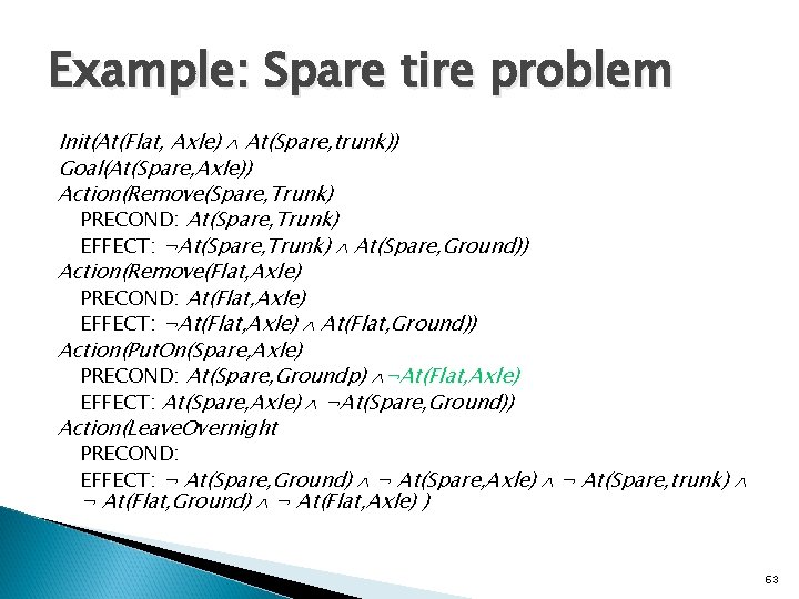
Example: Spare tire problem Init(At(Flat, Axle) At(Spare, trunk)) Goal(At(Spare, Axle)) Action(Remove(Spare, Trunk) PRECOND: At(Spare, Trunk) EFFECT: ¬At(Spare, Trunk) At(Spare, Ground)) Action(Remove(Flat, Axle) PRECOND: At(Flat, Axle) EFFECT: ¬At(Flat, Axle) At(Flat, Ground)) Action(Put. On(Spare, Axle) PRECOND: At(Spare, Groundp) ¬At(Flat, Axle) EFFECT: At(Spare, Axle) ¬At(Spare, Ground)) Action(Leave. Overnight PRECOND: EFFECT: ¬ At(Spare, Ground) ¬ At(Spare, Axle) ¬ At(Spare, trunk) ¬ At(Flat, Ground) ¬ At(Flat, Axle) ) 63

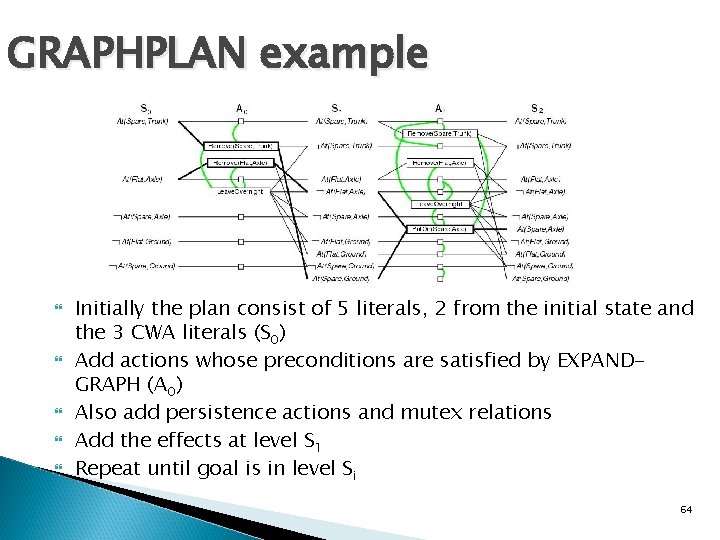
GRAPHPLAN example Initially the plan consist of 5 literals, 2 from the initial state and the 3 CWA literals (S 0) Add actions whose preconditions are satisfied by EXPANDGRAPH (A 0) Also add persistence actions and mutex relations Add the effects at level S 1 Repeat until goal is in level Si 64

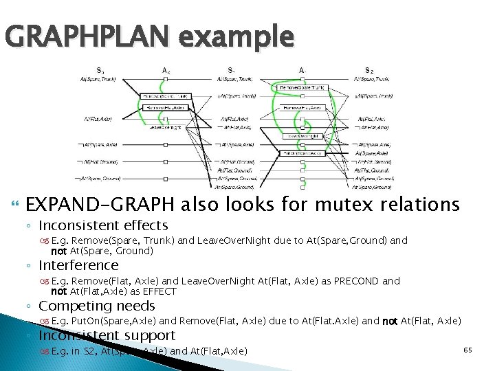
GRAPHPLAN example EXPAND-GRAPH also looks for mutex relations ◦ Inconsistent effects E. g. Remove(Spare, Trunk) and Leave. Over. Night due to At(Spare, Ground) and not At(Spare, Ground) ◦ Interference E. g. Remove(Flat, Axle) and Leave. Over. Night At(Flat, Axle) as PRECOND and not At(Flat, Axle) as EFFECT ◦ Competing needs E. g. Put. On(Spare, Axle) and Remove(Flat, Axle) due to At(Flat. Axle) and not At(Flat, Axle) ◦ Inconsistent support E. g. in S 2, At(Spare, Axle) and At(Flat, Axle) 65

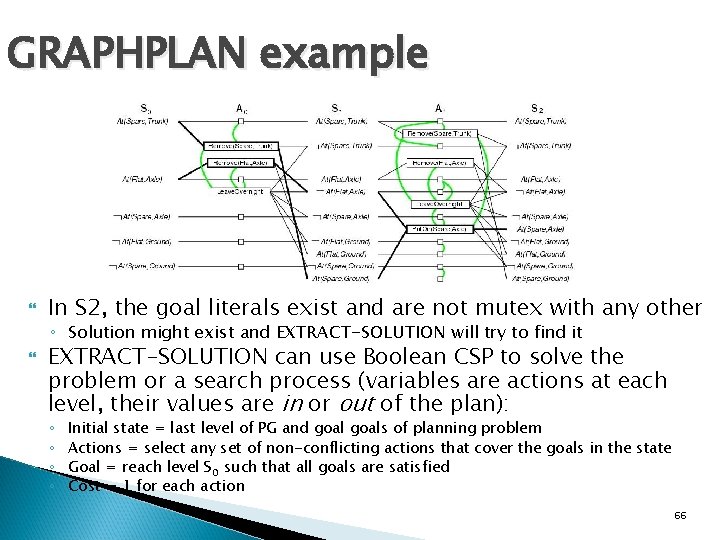
GRAPHPLAN example In S 2, the goal literals exist and are not mutex with any other ◦ Solution might exist and EXTRACT-SOLUTION will try to find it EXTRACT-SOLUTION can use Boolean CSP to solve the problem or a search process (variables are actions at each level, their values are in or out of the plan): ◦ ◦ Initial state = last level of PG and goals of planning problem Actions = select any set of non-conflicting actions that cover the goals in the state Goal = reach level S 0 such that all goals are satisfied Cost = 1 for each action 66

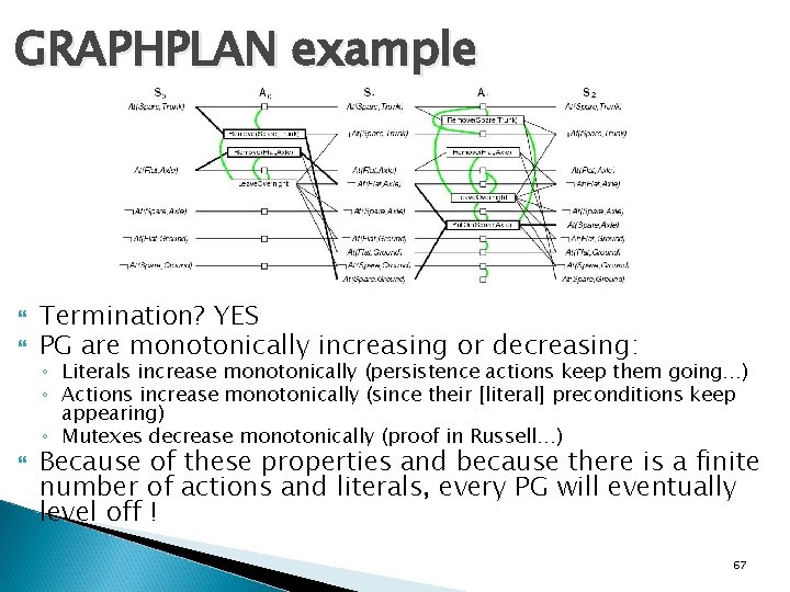
GRAPHPLAN example Termination? YES PG are monotonically increasing or decreasing: ◦ Literals increase monotonically (persistence actions keep them going…) ◦ Actions increase monotonically (since their [literal] preconditions keep appearing) ◦ Mutexes decrease monotonically (proof in Russell…) Because of these properties and because there is a finite number of actions and literals, every PG will eventually level off ! 67