Introduction to Artificial Intelligence AI Computer Science cpsc

Introduction to Artificial Intelligence (AI) Computer Science cpsc 502, Lecture 9 Oct, 11, 2011 Slide credit Approx. Inference : S. Thrun, P, Norvig, D. Klein CPSC 502, Lecture 9 Slide 1

Today Oct 11 • Bayesian Networks Approx. Inference • Temporal Probabilistic Models üMarkov Chains üHidden Markov Models CPSC 502, Lecture 9 2

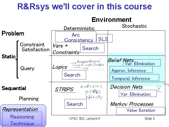
R&Rsys we'll cover in this course Environment Deterministic Problem Arc Consistency SLS Constraint Vars + Satisfaction Constraints Search Static Stochastic Belief Nets Query Logics Search Sequential Planning Representation Reasoning Technique STRIPS Search Var. Elimination Approx. Inference Temporal. Inference Decision Nets Var. Elimination Markov Processes Value Iteration CPSC 502, Lecture 9 Slide 3

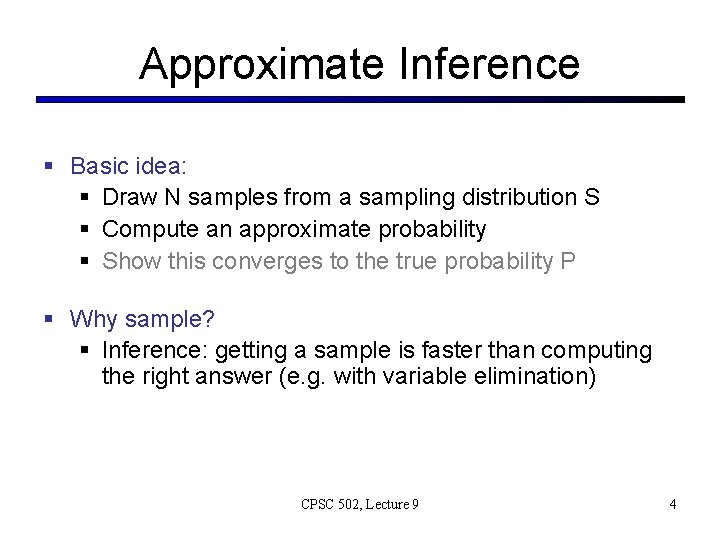
Approximate Inference § Basic idea: § Draw N samples from a sampling distribution S § Compute an approximate probability § Show this converges to the true probability P § Why sample? § Inference: getting a sample is faster than computing the right answer (e. g. with variable elimination) CPSC 502, Lecture 9 4

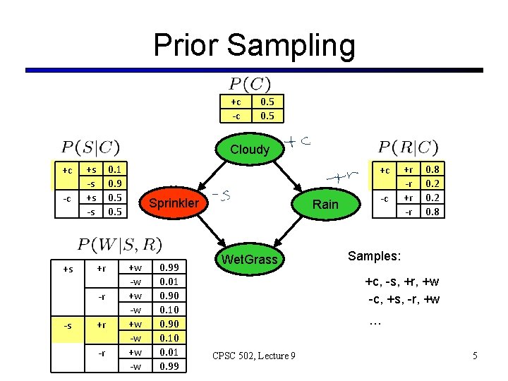
Prior Sampling +c -c 0. 5 Cloudy +c -c +s +s -s 0. 1 0. 9 0. 5 +r -r -s +r -r +c Sprinkler +w -w 0. 99 0. 01 0. 90 0. 10 0. 01 0. 99 Rain Wet. Grass -c +r -r 0. 8 0. 2 0. 8 Samples: +c, -s, +r, +w -c, +s, -r, +w … CPSC 502, Lecture 9 5

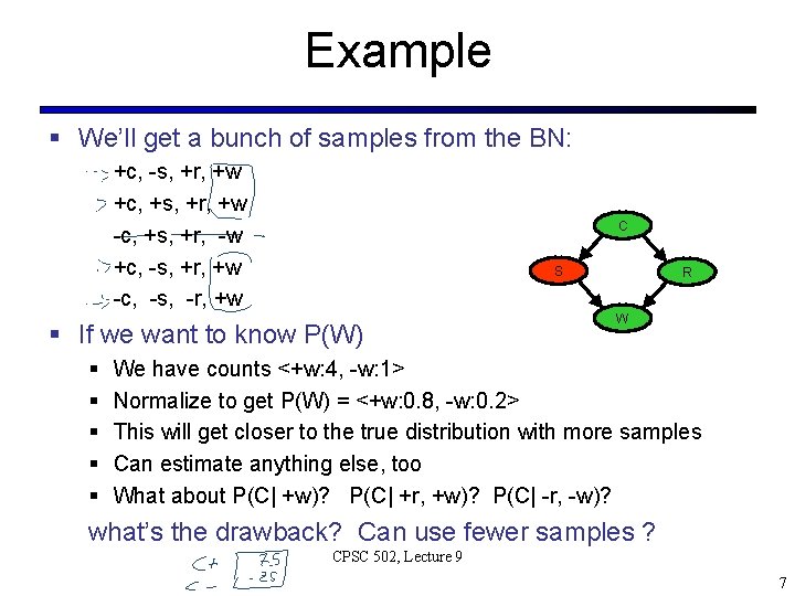
Example § We’ll get a bunch of samples from the BN: +c, -s, +r, +w +c, +s, +r, +w -c, +s, +r, -w +c, -s, +r, +w -c, -s, -r, +w Cloudy C Sprinkler S § If we want to know P(W) § § § Rain R Wet. Grass W We have counts <+w: 4, -w: 1> Normalize to get P(W) = <+w: 0. 8, -w: 0. 2> This will get closer to the true distribution with more samples Can estimate anything else, too What about P(C| +w)? P(C| +r, +w)? P(C| -r, -w)? what’s the drawback? Can use fewer samples ? CPSC 502, Lecture 9 7

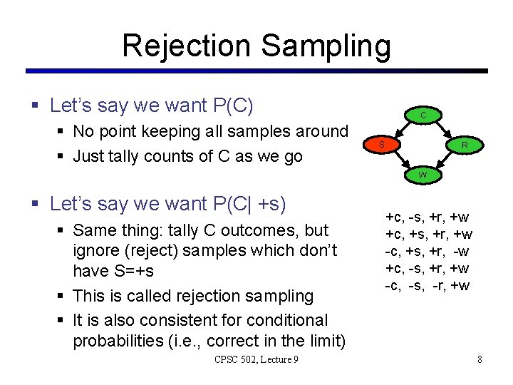
Rejection Sampling § Let’s say we want P(C) § No point keeping all samples around § Just tally counts of C as we go Cloudy C Sprinkler S Rain R Wet. Grass W § Let’s say we want P(C| +s) § Same thing: tally C outcomes, but ignore (reject) samples which don’t have S=+s § This is called rejection sampling § It is also consistent for conditional probabilities (i. e. , correct in the limit) CPSC 502, Lecture 9 +c, -s, +r, +w +c, +s, +r, +w -c, +s, +r, -w +c, -s, +r, +w -c, -s, -r, +w 8

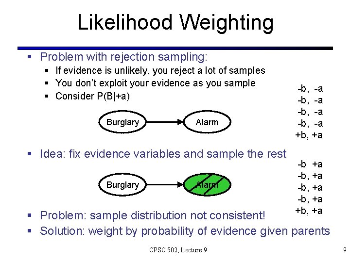
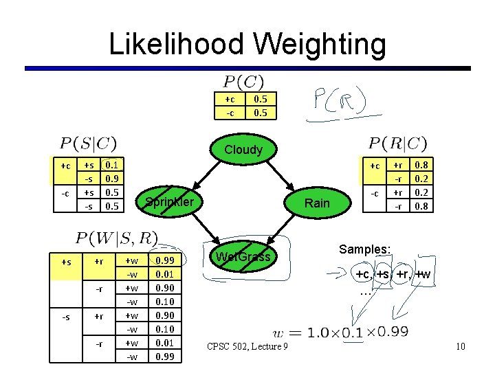
Likelihood Weighting § Problem with rejection sampling: § If evidence is unlikely, you reject a lot of samples § You don’t exploit your evidence as you sample § Consider P(B|+a) Burglary Alarm § Idea: fix evidence variables and sample the rest Burglary Alarm -b, -a +b, +a -b, +a +b, +a § Problem: sample distribution not consistent! § Solution: weight by probability of evidence given parents CPSC 502, Lecture 9 9

Likelihood Weighting +c -c 0. 5 Cloudy +c -c +s +s -s 0. 1 0. 9 0. 5 +r -r -s +r -r +c Sprinkler +w -w 0. 99 0. 01 0. 90 0. 10 0. 01 0. 99 Rain Wet. Grass -c +r -r 0. 8 0. 2 0. 8 Samples: +c, +s, +r, +w … CPSC 502, Lecture 9 10

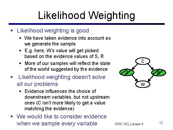
Likelihood Weighting § Likelihood weighting is good § We have taken evidence into account as we generate the sample § E. g. here, W’s value will get picked based on the evidence values of S, R § More of our samples will reflect the state of the world suggested by the evidence § Likelihood weighting doesn’t solve all our problems Cloudy C S Rain R W § Evidence influences the choice of downstream variables, but not upstream ones (C isn’t more likely to get a value matching the evidence) § We would like to consider evidence when we sample every variable CPSC 502, Lecture 9 12

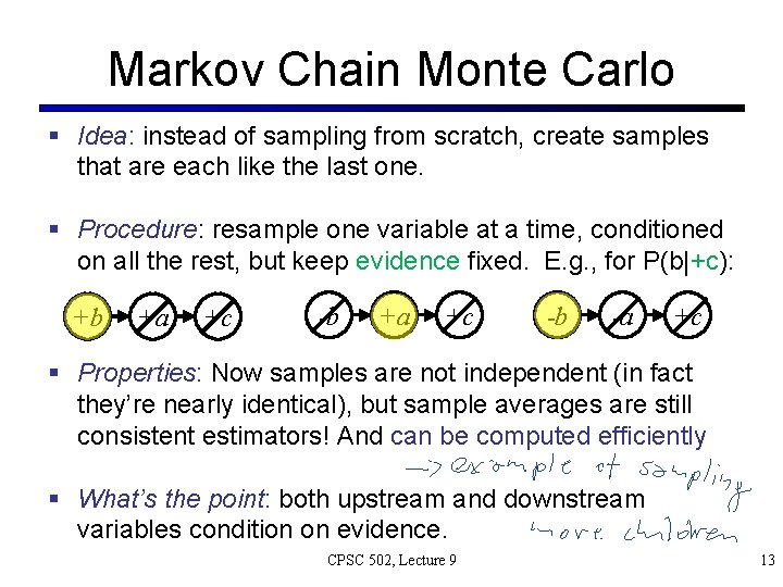
Markov Chain Monte Carlo § Idea: instead of sampling from scratch, create samples that are each like the last one. § Procedure: resample one variable at a time, conditioned on all the rest, but keep evidence fixed. E. g. , for P(b|+c): +b +a +c -b -a +c § Properties: Now samples are not independent (in fact they’re nearly identical), but sample averages are still consistent estimators! And can be computed efficiently § What’s the point: both upstream and downstream variables condition on evidence. CPSC 502, Lecture 9 13

Today Oct 11 § Bayesian Networks Approx. Inference § Temporal Probabilistic Models § Markov Chains § Hidden Markov Models CPSC 502, Lecture 9 14

Modelling static Environments So far we have used Bnets to perform inference in static environments • For instance, the system keeps collecting evidence to diagnose the cause of a fault in a system (e. g. , a car). • The environment (values of the evidence, the true cause) does not change as new evidence is gathered • What does change? The system’s beliefs over possible causes CPSC 502, Lecture 9 Slide 15

Modeling Evolving Environments: Dynamic Bnets • Often we need to make inferences about evolving environments. • Represent the state of the world at each specific point in time via a series of snapshots, or time slices, Solve. Problem t-1 Knows-Subtraction t-1 Solve. Problemt Knows-Subtraction t Morale t-1 Morale t Tutoring system tracing student knowledge and morale Slide 16 CPSC 502, Lecture 9

Today Oct 11 • Bayesian Networks Approx. Inference • Temporal Probabilistic Models üMarkov Chains üHidden Markov Models CPSC 502, Lecture 9 18

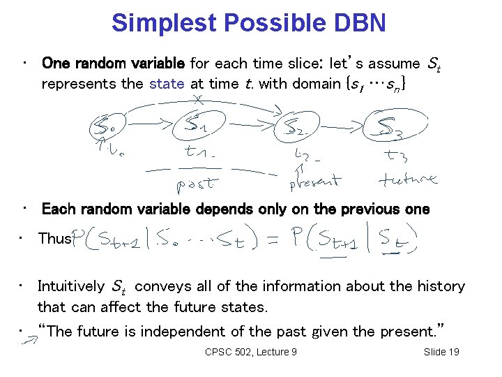
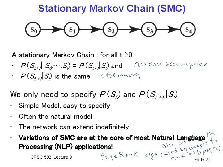
Simplest Possible DBN • One random variable for each time slice: let’s assume St represents the state at time t. with domain {s 1 …sn } • Each random variable depends only on the previous one • Thus • Intuitively St conveys all of the information about the history that can affect the future states. • “The future is independent of the past given the present. ” CPSC 502, Lecture 9 Slide 19

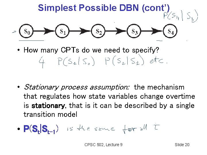
Simplest Possible DBN (cont’) • How many CPTs do we need to specify? • Stationary process assumption: the mechanism that regulates how state variables change overtime is stationary, that is it can be described by a single transition model • P(St|St-1) CPSC 502, Lecture 9 Slide 20

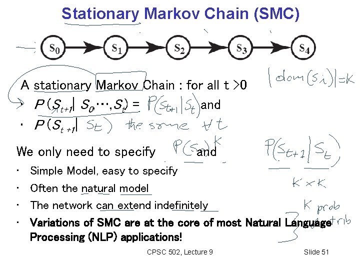
Stationary Markov Chain (SMC) A stationary Markov Chain : for all t >0 • P (St+1| S 0, …, St) = P (St+1|St) and • P (St +1|St) is the same We only need to specify P (S 0) and P (St +1 |St) • • Simple Model, easy to specify Often the natural model The network can extend indefinitely Variations of SMC are at the core of most Natural Language Processing (NLP) applications! CPSC 502, Lecture 9 Slide 21

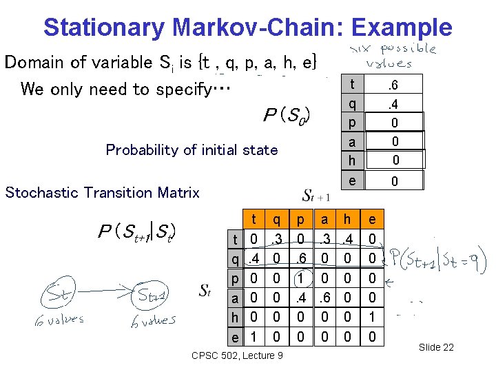
Stationary Markov-Chain: Example Domain of variable Si is {t , q, p, a, h, e} We only need to specify… P (S 0) Probability of initial state Stochastic Transition Matrix P (St+1|St) t q p a h e t 0. 4 0 0 0 1 t q p a h e q p a h. 3 0. 3. 4 0. 6 0 0 0 1 0 0 0. 4. 6 0 0 0 0 0 CPSC 502, Lecture 9 . 6. 4 0 0 e 0 0 1 0 Slide 22

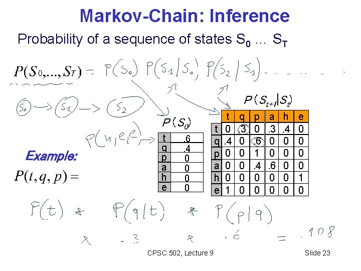
Markov-Chain: Inference Probability of a sequence of states S 0 … ST P (St+1|St) P (S 0) Example: t q p a h e . 6. 4 0 0 CPSC 502, Lecture 9 t q p a h e t 0. 4 0 0 0 1 q. 3 0 0 0 p 0. 6 1. 4 0 0 a. 3 0 0. 6 0 0 h. 4 0 0 0 e 0 0 1 0 Slide 23

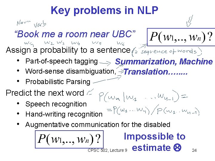
Key problems in NLP “Book me a room near UBC” Assign a probability to a sentence • Part-of-speech tagging Summarization, Machine • Word-sense disambiguation, Translation…. . . • Probabilistic Parsing Predict the next word • Speech recognition • Hand-writing recognition • Augmentative communication for the disabled Impossible to CPSC 502, Lecture 9 estimate 24

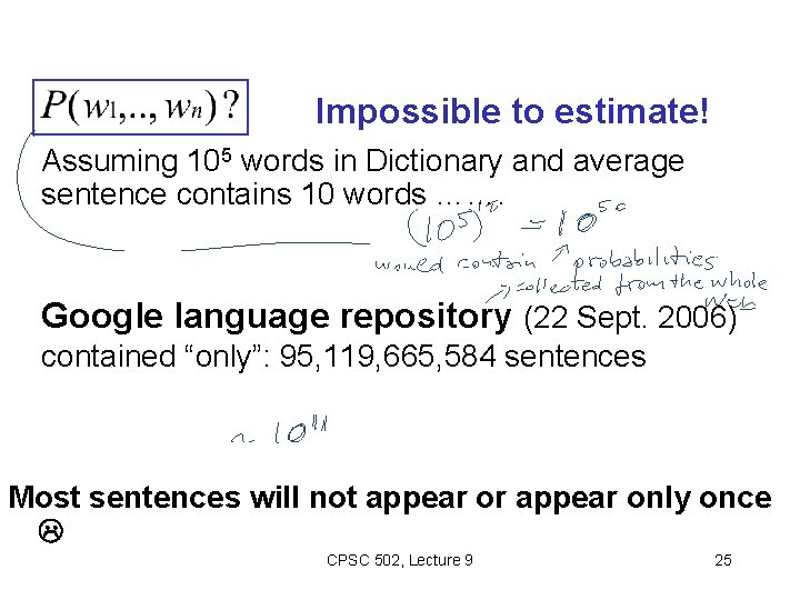
Impossible to estimate! Assuming 105 words in Dictionary and average sentence contains 10 words ……. Google language repository (22 Sept. 2006) contained “only”: 95, 119, 665, 584 sentences Most sentences will not appear or appear only once CPSC 502, Lecture 9 25

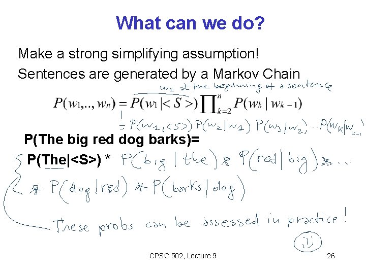
What can we do? Make a strong simplifying assumption! Sentences are generated by a Markov Chain P(The big red dog barks)= P(The|<S>) * CPSC 502, Lecture 9 26

Today Oct 11 • Bayesian Networks Approx. Inference • Temporal Probabilistic Models üMarkov Chains ü(Intro) Hidden Markov Models CPSC 502, Lecture 9 28

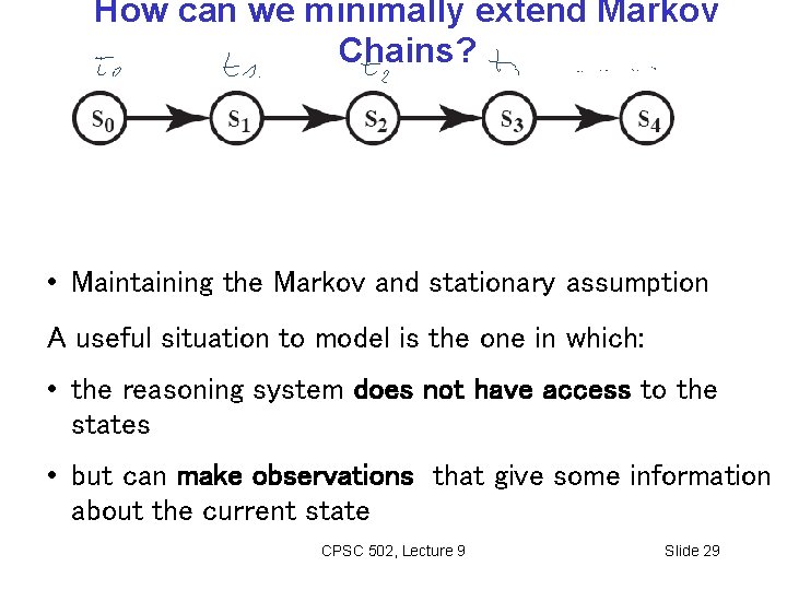
How can we minimally extend Markov Chains? • Maintaining the Markov and stationary assumption A useful situation to model is the one in which: • the reasoning system does not have access to the states • but can make observations that give some information about the current state CPSC 502, Lecture 9 Slide 29

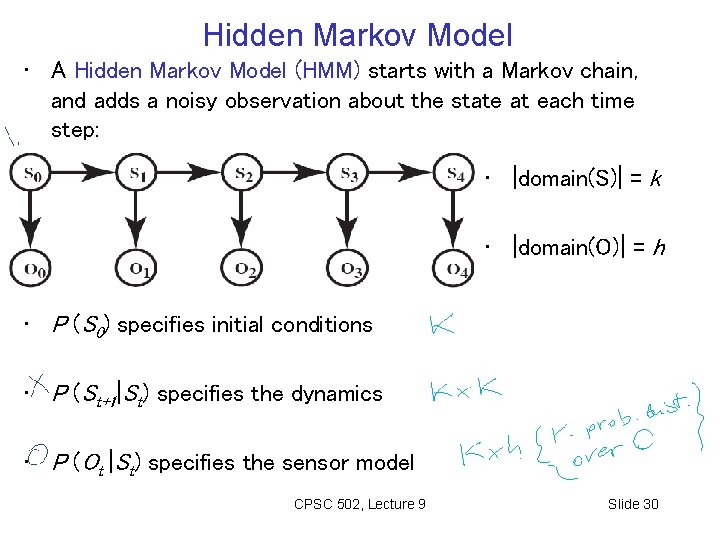
Hidden Markov Model • A Hidden Markov Model (HMM) starts with a Markov chain, and adds a noisy observation about the state at each time step: • |domain(S)| = k • |domain(O)| = h • P (S 0) specifies initial conditions • P (St+1|St) specifies the dynamics • P (Ot |St) specifies the sensor model CPSC 502, Lecture 9 Slide 30

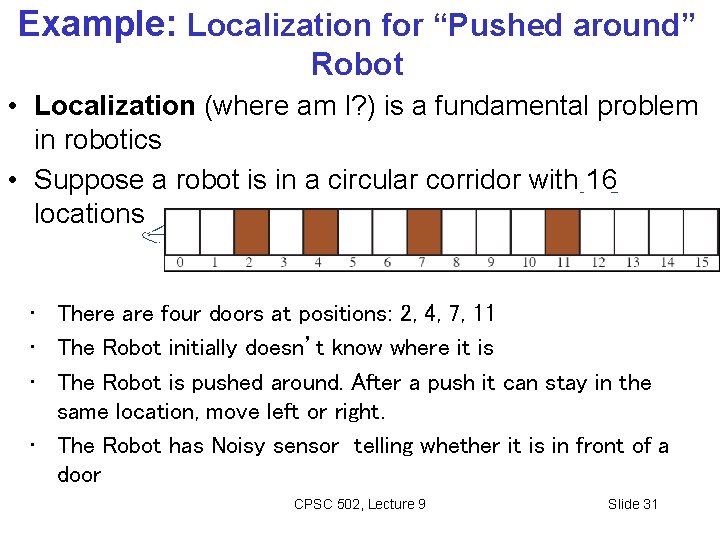
Example: Localization for “Pushed around” Robot • Localization (where am I? ) is a fundamental problem in robotics • Suppose a robot is in a circular corridor with 16 locations • There are four doors at positions: 2, 4, 7, 11 • The Robot initially doesn’t know where it is • The Robot is pushed around. After a push it can stay in the same location, move left or right. • The Robot has Noisy sensor telling whether it is in front of a door CPSC 502, Lecture 9 Slide 31

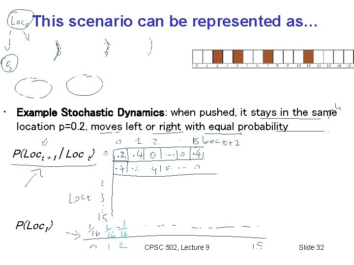
This scenario can be represented as… • Example Stochastic Dynamics: when pushed, it stays in the same location p=0. 2, moves left or right with equal probability P(Loct + 1 | Loc t) P(Loc 1) CPSC 502, Lecture 9 Slide 32

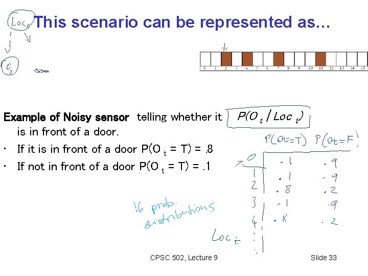
This scenario can be represented as… Example of Noisy sensor telling whether it is in front of a door. • If it is in front of a door P(O t = T) =. 8 • If not in front of a door P(O t = T) =. 1 CPSC 502, Lecture 9 P(O t | Loc t) Slide 33

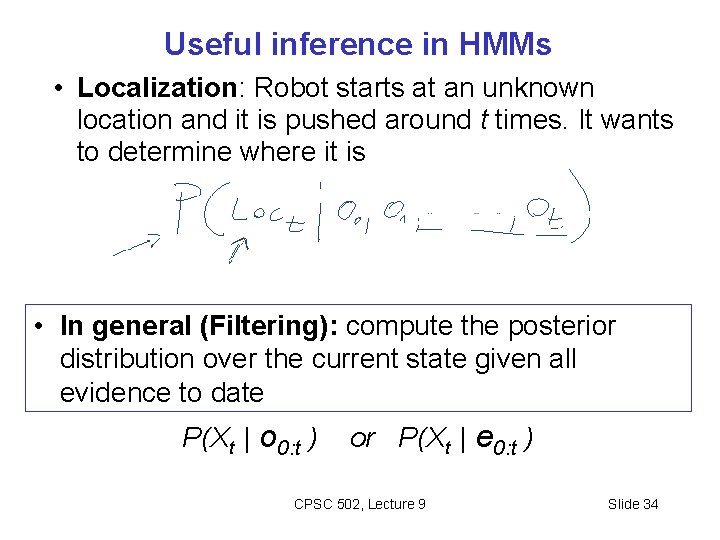
Useful inference in HMMs • Localization: Robot starts at an unknown location and it is pushed around t times. It wants to determine where it is • In general (Filtering): compute the posterior distribution over the current state given all evidence to date P(Xt | o 0: t ) or P(Xt | e 0: t ) CPSC 502, Lecture 9 Slide 34

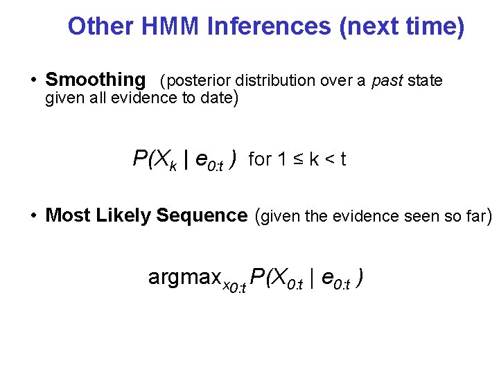
Other HMM Inferences (next time) • Smoothing (posterior distribution over a past state given all evidence to date) P(Xk | e 0: t ) for 1 ≤ k < t • Most Likely Sequence (given the evidence seen so far) argmaxx 0: t P(X 0: t | e 0: t )

TODO for this Thurs • Work on Assignment 2 • Study the Handout (on approx. inference) Available outside my office after 1 pm Also Do exercise 6. E (parts on importance sampling and particle filtering are optional) http: //www. aispace. org/exercises. shtml CPSC 502, Lecture 9 Slide 36

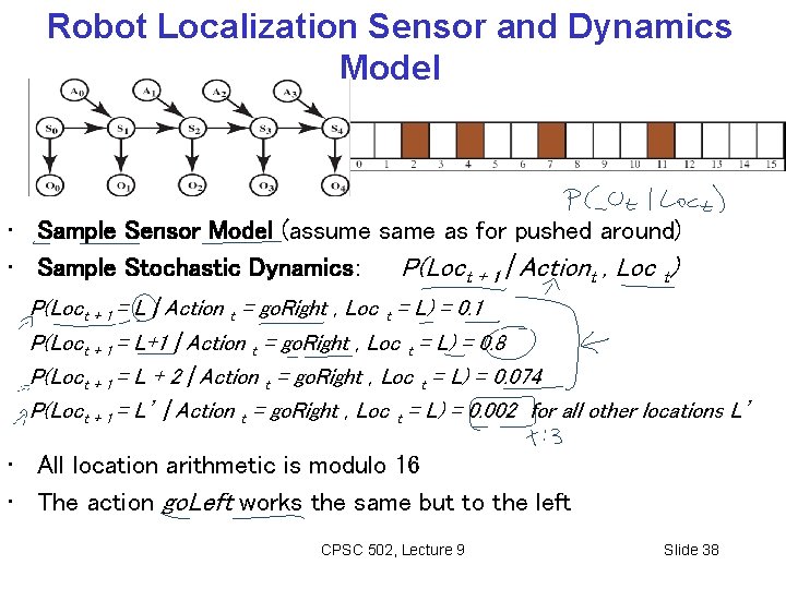
Example : Robot Localization • Suppose a robot wants to determine its location based on its actions and its sensor readings • Three actions: go. Right, go. Left, Stay • This can be represented by an augmented HMM CPSC 502, Lecture 9 Slide 37

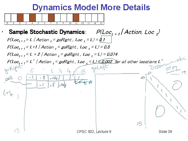
Robot Localization Sensor and Dynamics Model • Sample Sensor Model (assume same as for pushed around) • Sample Stochastic Dynamics: P(Loct + 1 | Actiont , Loc t) P(Loct + 1 = L | Action t = go. Right , Loc t = L) = 0. 1 P(Loct + 1 = L+1 | Action t = go. Right , Loc t = L) = 0. 8 P(Loct + 1 = L + 2 | Action t = go. Right , Loc t = L) = 0. 074 P(Loct + 1 = L’ | Action t = go. Right , Loc t = L) = 0. 002 for all other locations L’ • All location arithmetic is modulo 16 • The action go. Left works the same but to the left CPSC 502, Lecture 9 Slide 38

Dynamics Model More Details • Sample Stochastic Dynamics: P(Loct + 1 | Action, Loc t) P(Loct + 1 = L | Action t = go. Right , Loc t = L) = 0. 1 P(Loct + 1 = L+1 | Action t = go. Right , Loc t = L) = 0. 8 P(Loct + 1 = L + 2 | Action t = go. Right , Loc t = L) = 0. 074 P(Loct + 1 = L’ | Action t = go. Right , Loc t = L) = 0. 002 for all other locations L’ CPSC 502, Lecture 9 Slide 39

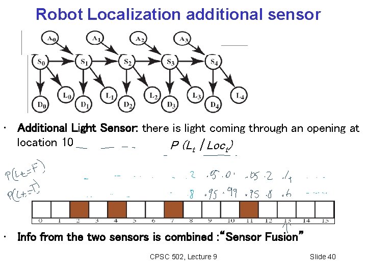
Robot Localization additional sensor • Additional Light Sensor: there is light coming through an opening at location 10 P (Lt | Loct) • Info from the two sensors is combined : “Sensor Fusion” CPSC 502, Lecture 9 Slide 40

The Robot starts at an unknown location and must determine where it is The model appears to be too ambiguous • Sensors are too noisy • Dynamics are too stochastic to infer anything But inference actually works pretty well. Let’s check: http: //www. cs. ubc. ca/spider/poole/demos/localization. html You can use standard Bnet inference. However you typically take advantage of the fact that time moves forward (not in 322) CPSC 502, Lecture 9 Slide 41

Sample scenario to explore in demo • Keep making observations without moving. What happens? • Then keep moving without making observations. What happens? • Assume you are at a certain position alternate moves and observations • …. CPSC 502, Lecture 9 Slide 42

HMMs have many other applications…. Natural Language Processing: e. g. , Speech Recognition • States: phoneme word • Bioinformatics: Observations: acoustic signal phoneme Gene Finding • States: coding / non-coding region • Observations: DNA Sequences For these problems the critical inference is: find the most likely sequence of states given a sequence of observations CPSC 502, Lecture 9 Slide 43

NEED to explain Filtering Because it will be used in POMDPs CPSC 502, Lecture 9 Slide 44

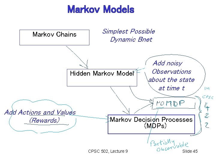
Markov Models Markov Chains Simplest Possible Dynamic Bnet Hidden Markov Model Add Actions and Values (Rewards) Add noisy Observations about the state at time t Markov Decision Processes (MDPs) CPSC 502, Lecture 9 Slide 45

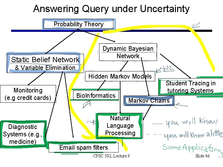
Answering Query under Uncertainty Probability Theory Static Belief Network Dynamic Bayesian Network & Variable Elimination Hidden Markov Models Monitoring (e. g credit cards) Diagnostic Systems (e. g. , medicine) Bio. Informatics Student Tracing in tutoring Systems Markov Chains Natural Language Processing Email spam filters CPSC 502, Lecture 9 Slide 46

Lecture Overview • Recap • Temporal Probabilistic Models • Start Markov Models § Markov Chains in Natural Language Processing CPSC 502, Lecture 9 Slide 47

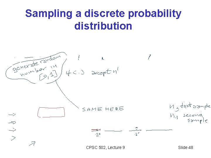
Sampling a discrete probability distribution CPSC 502, Lecture 9 Slide 48

Answering Query under Uncertainty Probability Theory Static Belief Network & Variable Elimination Monitoring (e. g credit cards) Diagnostic Systems (e. g. , medicine) Dynamic Bayesian Network Hidden Markov Models Bio. Informatic s Student Tracing in tutoring Systems Markov Chains Natural Language Processing Email spam filters CPSC 502, Lecture 9 Slide 49

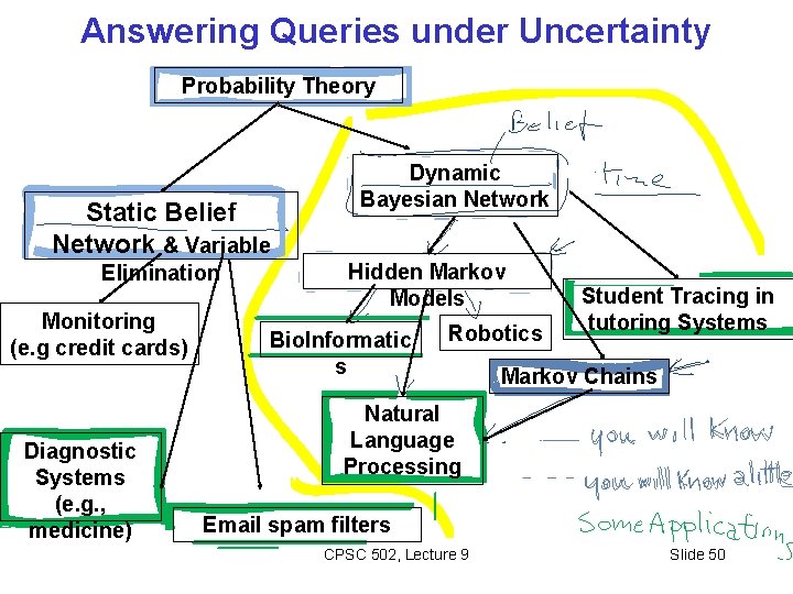
Answering Queries under Uncertainty Probability Theory Static Belief Network & Variable Elimination Monitoring (e. g credit cards) Diagnostic Systems (e. g. , medicine) Dynamic Bayesian Network Hidden Markov Models Bio. Informatic s Robotics Student Tracing in tutoring Systems Markov Chains Natural Language Processing Email spam filters CPSC 502, Lecture 9 Slide 50

Stationary Markov Chain (SMC) A stationary Markov Chain : for all t >0 • P (St+1| S 0, …, St) = and • P (St +1| We only need to specify • • and Simple Model, easy to specify Often the natural model The network can extend indefinitely Variations of SMC are at the core of most Natural Language Processing (NLP) applications! CPSC 502, Lecture 9 Slide 51