Introduction to Algorithms Syllabus 3 Sorting Specification Bubble

„Introduction to Algorithms“ Syllabus 3. Sorting – Specification – Bubble Sort – Selection Sort – Insertion Sort – Merge Sort – Quicksort – Linear-Time Median – Sorting in Linear Time – Sorting in Parallel Martin Ziegler • Specification • Primitives: semantics and cost • Design • Analysis • Optimality of Comparison-Based Sorting

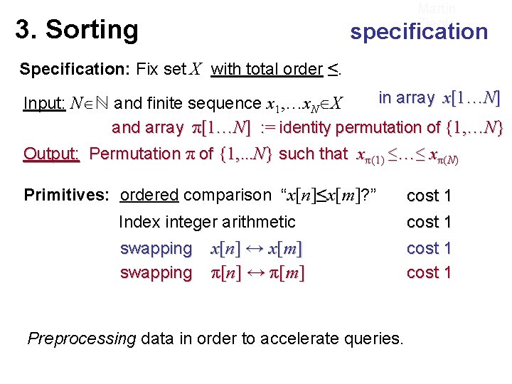
Martin Ziegler 3. Sorting specification Specification: Fix set X with total order ≤. in array x[1…N] Input: N ℕ and finite sequence x 1, …x. N X and array π[1…N] : = identity permutation of {1, …N} Output: Permutation π of x◦π {1, . . . such N} such Permuted array that xπ(1) x≤…≤ xπ(N) π(1) ≤…≤ Primitives: ordered comparison “x[n]≤x[m]? ” Index integer arithmetic swapping x[n] ↔ x[m] π[n] ↔ π[m] Preprocessing data in order to accelerate queries. cost 1

3. Sorting Martin Ziegler Bubble Sort Input: N ℕ and array x[1…N] Procedure Bubble. Sort ( x[N] ) For m : = N downto 2 do For k : = 1 to m− 1 do If x[k] > x[k+1] then Swap (x[k] , x[k+1]) Endif Output: Permuted array x◦π s. t. xπ(1) ≤…≤ xπ(N) Primitives: Comparison “x[n]≤x[m]? ” Swapping x[n] ↔ x[m] Index integer arithmetic Endfor runtime O(N²) Correctness: x[1], … x[m] ≤ x[m+1] ≤ … ≤ x[N]

3. Sorting Procedure Select. Sort ( x[N] ) For m : = 1 to N− 1 do min : = m; Martin Ziegler Select Sort Input: N ℕ and array x[1…N] Output: Permuted array x◦π s. t. xπ(1) ≤…≤ xπ(N) Primitives: For k : = min+1 to N do Comparison “x[n]≤x[m]? ” If x[k] < x[min] then Swapping x[n] ↔ x[m] Index integer arithmetic min : = k ; Endif Swap( x[m], x[min] ) Endfor runtime O(N²) Correctness: x[1] ≤ … ≤ x[m-1] ≤ x[m], … x[N]

3. Sorting Martin Ziegler Insert Sort Input: N ℕ and array x[1…N] Procedure Insert. Sort ( x[N] ) For m : = 2 to N do y : = x[m]; k : = m− 1; While k>0 and x[k]>y x[k+1] : = x[k] Output: Permuted array x◦π s. t. xπ(1) ≤…≤ xπ(N) Primitives: Comparison “x[n]≤x[m]? ” Swapping x[n] ↔ x[m] Index integer arithmetic k : = k − 1 Endwhile x[k+1] : = y Endfor runtime O(N²) Correctness: x[1] ≤ … ≤ x[m-1] ≤ x[m], … x[N]

Martin Ziegler 3. Sorting Procedure Merge. Sort ( x[N] ) Merge Sort Input: N ℕ and array x[1…N] Output: Permuted array x◦π s. t. xπ(1) ≤…≤ xπ(N) l : = N/2 ; r : = N/2 ; array y[l] , z[r] ; If N≤ 1 return. For m : = 1 to l do y[m]: = x[m]; For m : = 1 to r do z[m]: = x[l+m]; Merge. Sort(y); Merge. Sort(z); While l>0 and r>0 do ; If z[r] < y[l] then x[l+r] : = y[l] ; l: =l− 1 else x[l+r] : = z[r] ; r: =r− 1 runtime T(N) = 2·T(N/2) +O(N) ≤ O(N·log N) While l>0 do ; x[l+r] : = y[l] ; l: =l− 1 ; Endwhile While r>0 do ; x[l+r] : = z[r] ; r: =r− 1 ; Endwhile memory O(N·log N)

Martin Ziegler 3. Sorting Quick Sort Input: N ℕ and array x[1…N] Procedure Quick. Sort ( x[] ; l, r ) If l ≥ r return. // x[l]…x[r] sorted Output: Permuted array x◦π s. t. xπ(1) ≤…≤ xπ(N) samplepivot s : = xx[[ rl]; (]; l+r)/2 ]]; XX ////sample T (N ) ≤ O (N ) + a : = l ; b : = r ; While a < b do ++ TT((N -2) ++ TT(1) (2) N-1) While a<b and x[a] < s do a : = a+1 Endwhile; = O(N²) While a<b and x[b] ≥ s do b : = b-1 Endwhile; Swap(x[a], x[b]); Endwhile ; l a=b r // l ≤ a = b ≤ r Quick. Sort ( x , l , a-1); Quick. Sort ( x , b+1 , r); Idea: s: =x[p] for random p [l. . r] Quick. Sort is in worst-case as bad as Bubble. Sort → randomized algorithms

3. Sorting Martin Ziegler continued: Quick Sort Input: N ℕ and array x[1…N] Procedure Quick. Sort ( x[] ; l, r ) Output: Permuted array x◦π If l ≥ r return. // x([lx]… Function Partition [] ; xl[r, ]r sorted ; y) s. t. xπ(1) ≤…≤ xπ(N) // splits x[l. . r]: into x [ l. . m ] with entries < y samplepivot s : = xx[[ rl]; (]; l+r)/2 ]]; XX ////sample T(N) = T(N· ε? ) // and x[m+1. . r] those ≥y. Returns m. a : = l ; b : = r ; While a < b do + T(N·(1− ε? )) +O(N) While a<b and x[a] < y do a : = a+1 Endwhile; ≤ O(N·log N) While a<b and x[b] ≥ y do b : = b-1 Endwhile; if (0, 1) fixed Swap(x[a], x[b]); Endwhile ; Return // l ≤ aa; = b ≤ r l a=b r ε·(r-l+1) ≤ a−l ≤ (1 -ε)·(r-l+1) Quick. Sort ( x , l , a-1); ε·(r-l+1) ≤ r−a ≤ (1 -ε)·(r-l+1) Quick. Sort ( x , b+1 , r); c·N·log(N) =: T(N) = c·N· ·log(N· ) + c·N·(1 - )·log(N·(1 - )) + N = c·N·log(N) + N·c·( ·log( ) + (1 - )·log(1 - )) + N Ansatz

3. Sorting Martin Ziegler Median Revisited Function Partition ( x[] ; l , r ; s) Input: N ℕ and array x[1…N] // splits x[l. . r]: into x[l. . m] with entries <s W. l. o. g. x[n]≠x[m] for all n≠m // and x[m+1. . r] those ≥s. Returns m. K-th order statistic: m s. t. #{n : xn<xm} < K ≤ #{n : xn≤xm} ε·(r-l+1)M≤edian a−l of ≤ (1ε)·(r-l+1) Lemma: 5 -medians isε·(“≤ at least 30% r-”l+1) ≤ r−½·⅗ a ≤=(1ε)·(of r-l+1) entries, and “>“ at most 70%. Output: m such that 0. 3·N ≤ #{n : xn ≤ xm } ≤ 0. 7·N+1

Martin Ziegler 3. Sorting Linear-time Median Function Partition ( x[] ; l , r ; y) // partitions x[l. . r] into x[l. . m] entries <y // and x[m+1. . r] those ≥y. Returns m. Function Order. Stat ( x[] ; l, r , K) While l<r do Call Approx. Med in order to determine an approximate median s of x[l…r]. Partition x[l…r] accordingly. Proceed to the left (=decrease r) /right (=increase l) accordingly. K-th order statistic: m s. t. #{n : xn<xm} < K ≤ #{n : xn≤xm} TA(n) = O(n) + TO(0. 2·n) , Input: N ℕ and array x[1…N] W. l. o. g. x[n]≠x[m] for all n≠m Function Approx. Med ( x[] ; l , r) Process x[l. . . r] in groups of 5: For each group, find its median (for instance by brute force). Then call Order. Stat to determine the median of these 5 medians. n : = r − l+1 Lemma: Median of 5 -medians is “≤” at least ½·⅗ = 30% of entries, and “>“ at most 70%. TO(n) = TA(n) + O(n) + TO(0. 7·n)

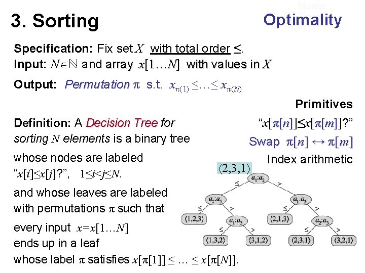
Martin Ziegler 3. Sorting Optimality Specification: Fix set X with total order ≤. Input: N ℕ and array x[1…N] with values in X Output: Permutation π s. t. xπ(1) ≤…≤ xπ(N) Primitives Definition: A Decision Tree for sorting N elements is a binary tree whose nodes are labeled “x[i]≤x[j]? ”, 1≤i<j≤N. “x[π[n]]≤x[π[m]]? ” Swap π[n] ↔ π[m] Index arithmetic 2, 3, 1 and whose leaves are labeled with permutations π such that every input x=x[1…N] ends up in a leaf whose label π satisfies x[π[1]] ≤ … ≤ x[π[N]].

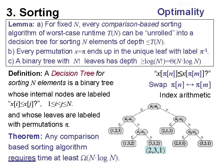
3. Sorting Martin Ziegler Optimality Lemma: a) For fixed N, every comparison-based sorting algorithm of worst-case runtime T(N) can be “unrolled” into a decision tree for sorting N elements of depth ≤T(N). b) Every permutation x=π ends up in the unique leaf with label π-1. c) A binary tree with N! leaves has depth ≥log(N!)=Θ(N·log N) Definition: A Decision Tree for sorting N elements is a binary tree whose internal nodes are labeled “x[i]≤x[j]? ”, 1≤i<j≤N. “x[π[n]]≤x[π[m]]? ” Swap π[n] ↔ π[m] Index arithmetic and whose leaves are labeled with permutations ππ. such that every input Any x=x[1…N] Theorem: comparison ends in a leaf basedupsorting algorithm 2, 3, 1 whose label π satisfies ≤ …N≤ requires time at least x[π[1]] Ω(N·log ). x[π[N]].

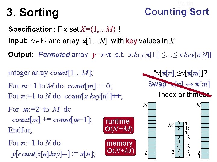
Martin Ziegler 3. Sorting Counting Sort Specification: Fix set X={1, …M} ! Input: N ℕ and array x[1…N] with key values in X Output: Permuted array y=x◦π s. t. x. key[π[1]] ≤…≤ x. key[π[N]] integer array count[1…M]; “x[π[n]]≤x[π[m]]? ” Swap π[n] ↔ π[m] Index arithmetic For m: =1 to M do count[m] : = 0; For n: =1 to N do count[x. key[n]]++; For m: =2 to M do count[m] += count[m− 1]; Endfor; For n: =1 to N do y[count[x[n]. key]--] : = x[n]; N runtime N M O(N+M) memory O (N + M) 2 1 0 15 5 15 1 10 0 9 4 9 2 5 3 3 2 1

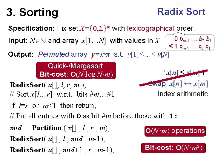
3. Sorting Martin Ziegler Radix Sort Specification: Fix set X={0, 1}m with lexicographical order. Input: N ℕ and array x[1…N] with values in X 0 bm-1 … b 2 b 1 < 1 cm-1 … c 2 c 1 Output: Permuted array y=x◦π s. t. y[1] ≤…≤ y[N] Quick-/Mergesort Bit-cost: O(N·log N·m) “x[n] ≤ x[m] ? ” Swap x[n] ↔ x[m] Radix. Sort( x[], l, r, m ); Index arithmetic // Sort x[l…r] w. r. t. bits #m…#1 If l=r or m<1 then return; // Put all entries with 0 as bit #m before those with 1: mid : = Partition ( x[] , l , r , m); Radix. Sort( x[] , l , mid , m-1); Radix. Sort( x[] , mid+1 , r , m-1); O(N·m) operations Bit-cost: O(N·m²)

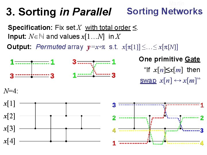
3. Sorting in Parallel Martin Ziegler Sorting Networks Specification: Fix set X with total order ≤. Input: N ℕ and values x[1…N] in X Output: Permuted array y=x◦π s. t. x[π[1]] ≤…≤ x[π[N]] One primitive Gate “If x[n]≤x[m] then swap x[n] ↔ x[m]” N=4: x[1] x[2] x[3] x[4]

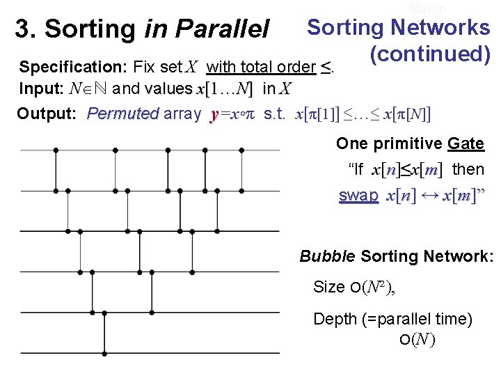
Martin Ziegler 3. Sorting in Parallel Sorting Networks (continued) with total order ≤. Specification: Fix set X Input: N ℕ and values x[1…N] in X Output: Permuted array y=x◦π s. t. x[π[1]] ≤…≤ x[π[N]] One primitive Gate “If x[n]≤x[m] then swap x[n] ↔ x[m]” Bubble Sorting Network: Size O(N²), Depth (=parallel time) O(N)

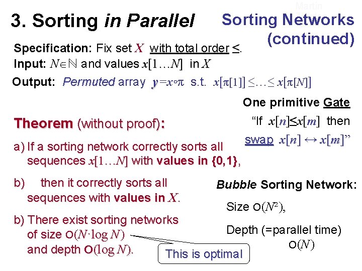
Martin Ziegler 3. Sorting in Parallel Sorting Networks (continued) with total order ≤. Specification: Fix set X Input: N ℕ and values x[1…N] in X Output: Permuted array y=x◦π s. t. x[π[1]] ≤…≤ x[π[N]] One primitive Gate “If x[n]≤x[m] then Theorem (without proof): a) If a sorting network correctly sorts all sequences x[1…N] with values in {0, 1}, b) then it correctly sorts all sequences with values in X. swap x[n] ↔ x[m]” Bubble Sorting Network: Size O(N²), b) There exist sorting networks Depth (=parallel time) of size O(N·log N) O(N) and depth O(log N). This is optimal

„Introduction to Algorithms“ Summary 3. Sorting – Specification – Bubble Sort – Selection Sort – Insertion Sort – Merge Sort – Quicksort – Linear-Time Median – Sorting in Linear Time – Sorting in Parallel Martin Ziegler • Specification • Primitives: semantics and cost • Design • Analysis • Optimality of Comparison-Based Sorting