Introduction to Algorithms Sorting in Linear Time CSE

Introduction to Algorithms Sorting in Linear Time CSE 680 Prof. Roger Crawfis

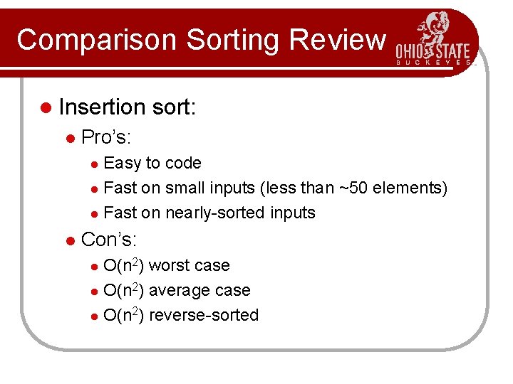
Comparison Sorting Review l Insertion l sort: Pro’s: Easy to code l Fast on small inputs (less than ~50 elements) l Fast on nearly-sorted inputs l l Con’s: O(n 2) worst case l O(n 2) average case l O(n 2) reverse-sorted case l

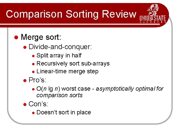
Comparison Sorting Review l Merge l sort: Divide-and-conquer: Split array in half l Recursively sort sub-arrays l Linear-time merge step l l Pro’s: l l O(n lg n) worst case - asymptotically optimal for comparison sorts Con’s: l Doesn’t sort in place

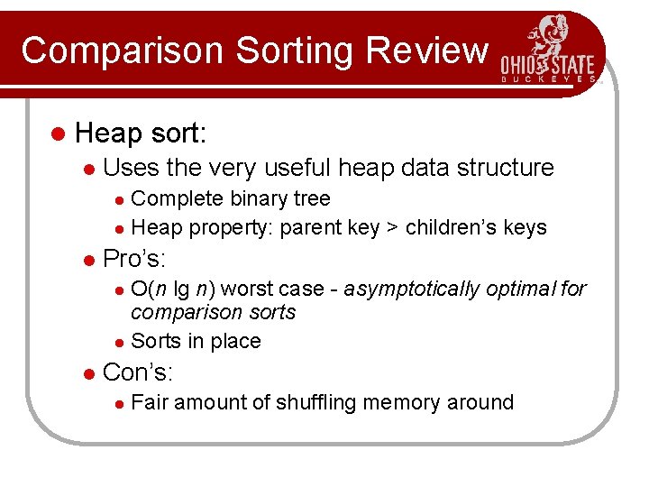
Comparison Sorting Review l Heap l sort: Uses the very useful heap data structure Complete binary tree l Heap property: parent key > children’s keys l l Pro’s: O(n lg n) worst case - asymptotically optimal for comparison sorts l Sorts in place l l Con’s: l Fair amount of shuffling memory around

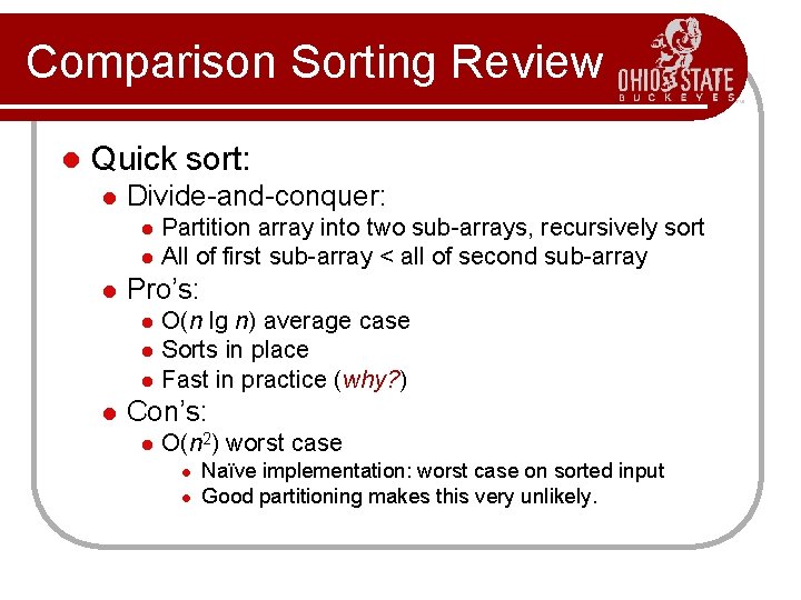
Comparison Sorting Review l Quick sort: l Divide-and-conquer: l l l Pro’s: l l Partition array into two sub-arrays, recursively sort All of first sub-array < all of second sub-array O(n lg n) average case Sorts in place Fast in practice (why? ) Con’s: l O(n 2) worst case l l Naïve implementation: worst case on sorted input Good partitioning makes this very unlikely.

Non-Comparison Based Sorting l Many times we have restrictions on our keys l l Deck of cards: Ace->King and four suites Social Security Numbers Employee ID’s We will examine three algorithms which under certain conditions can run in O(n) time. l l l Counting sort Radix sort Bucket sort

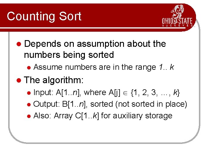
Counting Sort l Depends on assumption about the numbers being sorted l Assume numbers are in the range 1. . k l The algorithm: Input: A[1. . n], where A[j] {1, 2, 3, …, k} l Output: B[1. . n], sorted (not sorted in place) l Also: Array C[1. . k] for auxiliary storage l

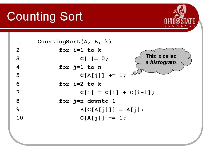
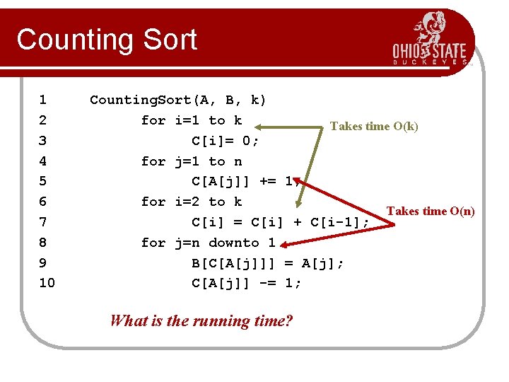
Counting Sort 1 2 3 4 5 6 7 8 9 10 Counting. Sort(A, B, k) for i=1 to k This is called C[i]= 0; a histogram. for j=1 to n C[A[j]] += 1; for i=2 to k C[i] = C[i] + C[i-1]; for j=n downto 1 B[C[A[j]]] = A[j]; C[A[j]] -= 1;

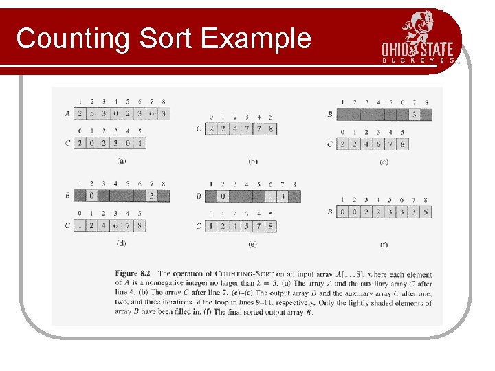
Counting Sort Example

Counting Sort 1 2 3 4 5 6 7 8 9 10 Counting. Sort(A, B, k) for i=1 to k Takes time O(k) C[i]= 0; for j=1 to n C[A[j]] += 1; for i=2 to k Takes time O(n) C[i] = C[i] + C[i-1]; for j=n downto 1 B[C[A[j]]] = A[j]; C[A[j]] -= 1; What is the running time?

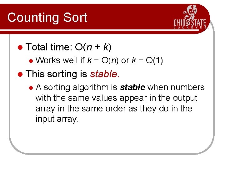
Counting Sort l Total l Works well if k = O(n) or k = O(1) l This l time: O(n + k) sorting is stable. A sorting algorithm is stable when numbers with the same values appear in the output array in the same order as they do in the input array.

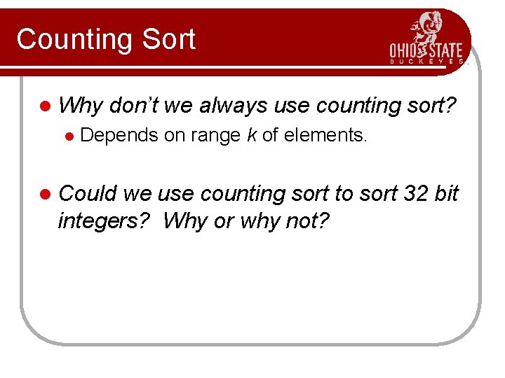
Counting Sort l Why l don’t we always use counting sort? Depends on range k of elements. l Could we use counting sort to sort 32 bit integers? Why or why not?

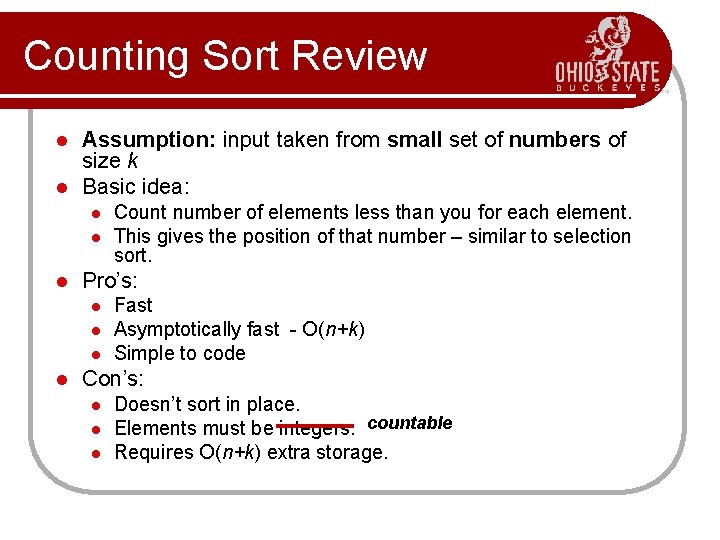
Counting Sort Review Assumption: input taken from small set of numbers of size k l Basic idea: l l Pro’s: l l Count number of elements less than you for each element. This gives the position of that number – similar to selection sort. Fast Asymptotically fast - O(n+k) Simple to code Con’s: l l l Doesn’t sort in place. Elements must be integers. countable Requires O(n+k) extra storage.

Radix Sort l How did IBM get rich originally? l Answer: punched card readers for census tabulation in early 1900’s. l In particular, a card sorter that could sort cards into different bins Each column can be punched in 12 places l Decimal digits use 10 places l l Problem: only one column can be sorted on at a time

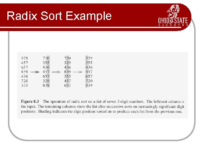
Radix Sort Intuitively, you might sort on the most significant digit, then the second msd, etc. l Problem: lots of intermediate piles of cards (read: scratch arrays) to keep track of l Key idea: sort the least significant digit first l Radix. Sort(A, d) for i=1 to d Stable. Sort(A) on digit i

Radix Sort Example

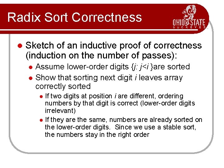
Radix Sort Correctness l Sketch of an inductive proof of correctness (induction on the number of passes): l l Assume lower-order digits {j: j<i }are sorted Show that sorting next digit i leaves array correctly sorted l l If two digits at position i are different, ordering numbers by that digit is correct (lower-order digits irrelevant) If they are the same, numbers are already sorted on the lower-order digits. Since we use a stable sort, the numbers stay in the right order

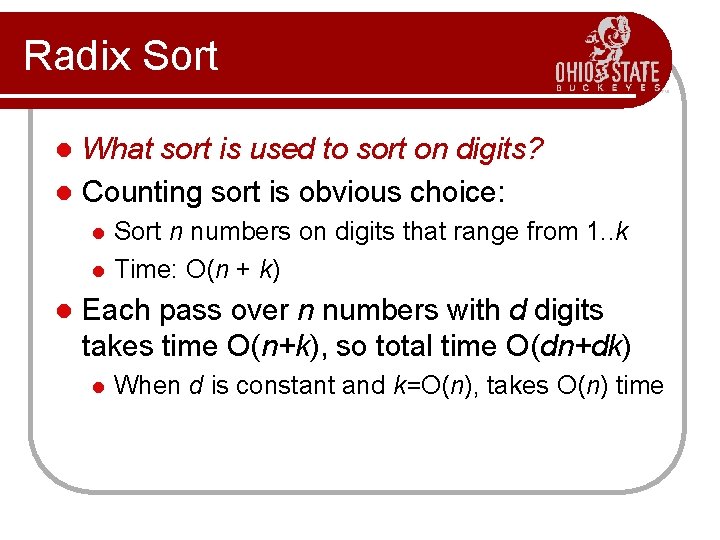
Radix Sort What sort is used to sort on digits? l Counting sort is obvious choice: l l Sort n numbers on digits that range from 1. . k Time: O(n + k) Each pass over n numbers with d digits takes time O(n+k), so total time O(dn+dk) l When d is constant and k=O(n), takes O(n) time

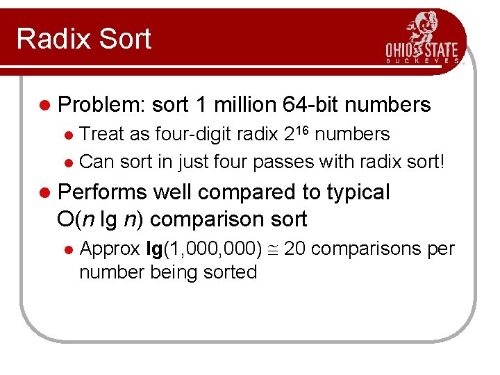
Radix Sort l Problem: sort 1 million 64 -bit numbers Treat as four-digit radix 216 numbers l Can sort in just four passes with radix sort! l l Performs well compared to typical O(n lg n) comparison sort l Approx lg(1, 000) 20 comparisons per number being sorted

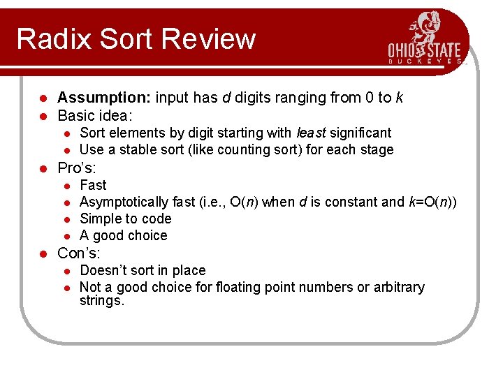
Radix Sort Review l l Assumption: input has d digits ranging from 0 to k Basic idea: l l l Pro’s: l l l Sort elements by digit starting with least significant Use a stable sort (like counting sort) for each stage Fast Asymptotically fast (i. e. , O(n) when d is constant and k=O(n)) Simple to code A good choice Con’s: l l Doesn’t sort in place Not a good choice for floating point numbers or arbitrary strings.

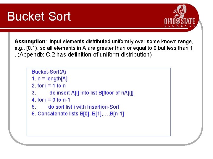
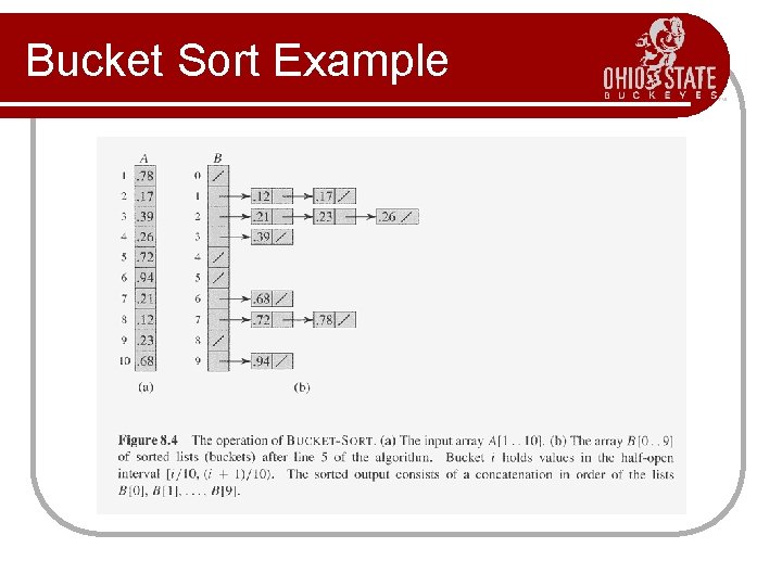
Bucket Sort Assumption: input elements distributed uniformly over some known range, e. g. , [0, 1), so all elements in A are greater than or equal to 0 but less than 1. (Appendix C. 2 has definition of uniform distribution) Bucket-Sort(A) 1. n = length[A] 2. for i = 1 to n 3. do insert A[i] into list B[floor of n. A[i]] 4. for i = 0 to n-1 5. do sort list i with Insertion-Sort 6. Concatenate lists B[0], B[1], …, B[n-1]

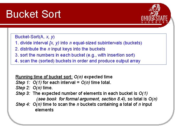
Bucket Sort Bucket-Sort(A, x, y) 1. divide interval [x, y) into n equal-sized subintervals (buckets) 2. distribute the n input keys into the buckets 3. sort the numbers in each bucket (e. g. , with insertion sort) 4. scan the (sorted) buckets in order and produce output array Running time of bucket sort: O(n) expected time Step 1: O(1) for each interval = O(n) time total. Step 2: O(n) time. Step 3: The expected number of elements in each bucket is O(1) (see book formal argument, section 8. 4), so total is O(n) Step 4: O(n) time to scan the n buckets containing a total of n input elements

Bucket Sort Example

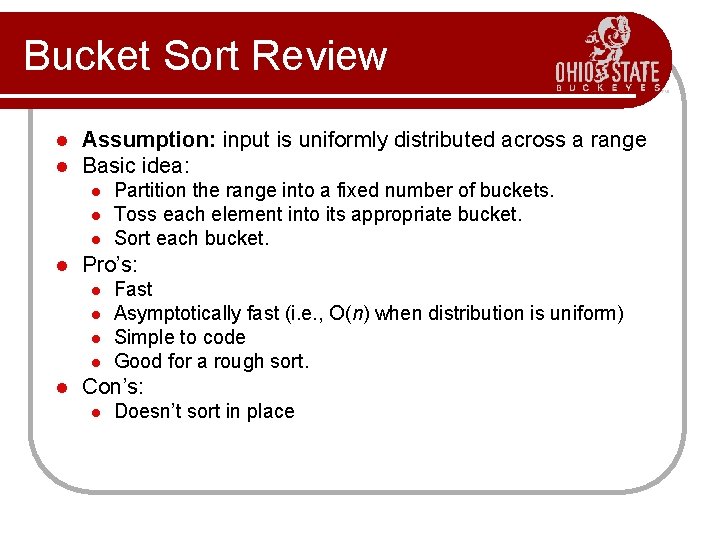
Bucket Sort Review l l Assumption: input is uniformly distributed across a range Basic idea: l l Pro’s: l l l Partition the range into a fixed number of buckets. Toss each element into its appropriate bucket. Sort each bucket. Fast Asymptotically fast (i. e. , O(n) when distribution is uniform) Simple to code Good for a rough sort. Con’s: l Doesn’t sort in place

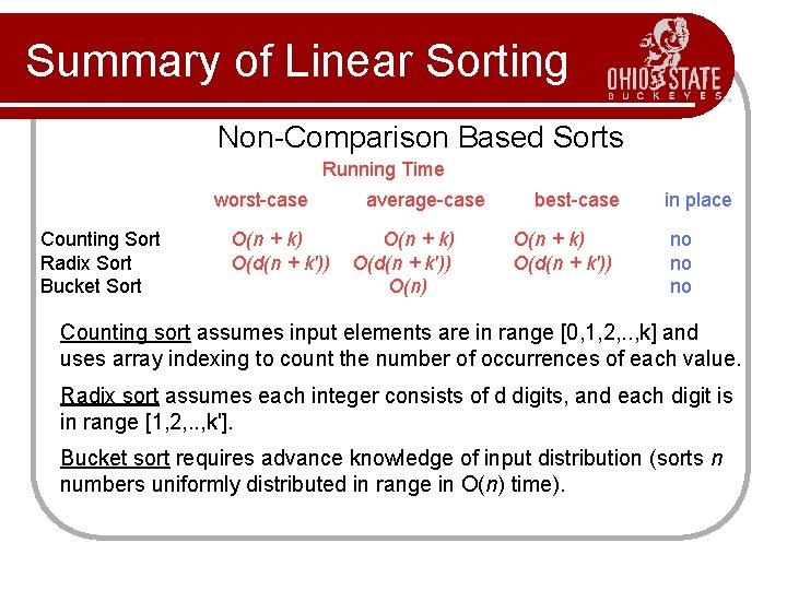
Summary of Linear Sorting Non-Comparison Based Sorts Running Time worst-case Counting Sort Radix Sort Bucket Sort O(n + k) O(d(n + k')) average-case O(n + k) O(d(n + k')) O(n) best-case O(n + k) O(d(n + k')) in place no no no Counting sort assumes input elements are in range [0, 1, 2, . . , k] and uses array indexing to count the number of occurrences of each value. Radix sort assumes each integer consists of d digits, and each digit is in range [1, 2, . . , k']. Bucket sort requires advance knowledge of input distribution (sorts n numbers uniformly distributed in range in O(n) time).