Introduction to Algorithms Dynamic Programming Introduction to Algorithms

Introduction to Algorithms: Dynamic Programming

Introduction to Algorithms Dynamic Programming • Longest common subsequence • Optimal substructure • Overlapping subproblems CS 421 - Introduction to Algorithms 2

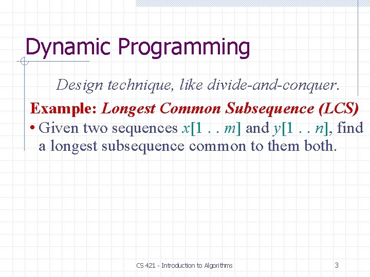
Dynamic Programming Design technique, like divide-and-conquer. Example: Longest Common Subsequence (LCS) • Given two sequences x[1. . m] and y[1. . n], find a longest subsequence common to them both. CS 421 - Introduction to Algorithms 3

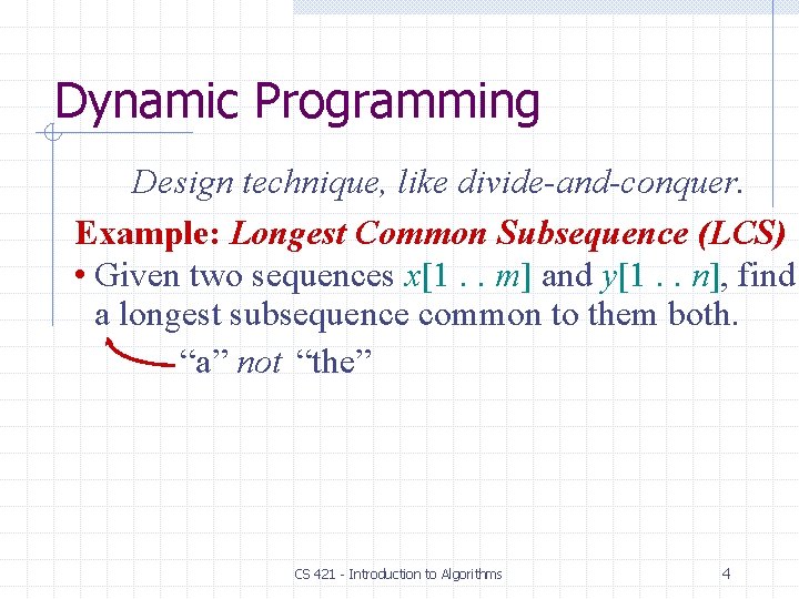
Dynamic Programming Design technique, like divide-and-conquer. Example: Longest Common Subsequence (LCS) • Given two sequences x[1. . m] and y[1. . n], find a longest subsequence common to them both. “a” not “the” CS 421 - Introduction to Algorithms 4

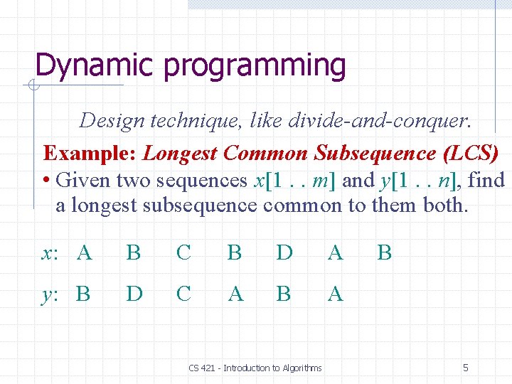
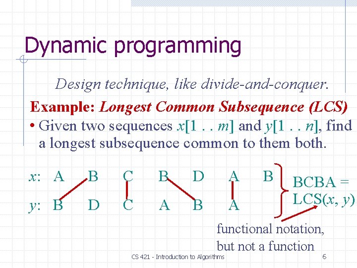
Dynamic programming Design technique, like divide-and-conquer. Example: Longest Common Subsequence (LCS) • Given two sequences x[1. . m] and y[1. . n], find a longest subsequence common to them both. x: A B C B D A y: B D C A B A CS 421 - Introduction to Algorithms B 5

Dynamic programming Design technique, like divide-and-conquer. Example: Longest Common Subsequence (LCS) • Given two sequences x[1. . m] and y[1. . n], find a longest subsequence common to them both. x: A B C B D A y: B D C A B BCBA = LCS(x, y) functional notation, but not a function CS 421 - Introduction to Algorithms 6

Brute-Force LCS Algorithm Check every subsequence of x[1. . m] to see if it is also a subsequence of y[1. . n]. Check if str 1 is a substring of str 2 is. Sub. Sequence(str 1, str 2, m, n): j = 0 # Index of str 1 i = 0 # Index of str 2 while j<m and i<n: if str 1[j] == str 2[i]: j = j+1 i=i+1 return j==m CS 421 - Introduction to Algorithms 7

Brute-Force LCS Algorithm Check every subsequence of x[1. . m] to see if it is also a subsequence of y[1. . n]. Analysis Checking = O(n) time per subsequence. 2 m subsequences of x (each bit-vector of length m determines a distinct subsequence of x). Worst-case running time = O(n 2 m) = exponential time. CS 421 - Introduction to Algorithms 8

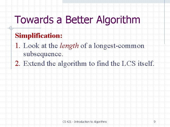
Towards a Better Algorithm Simplification: 1. Look at the length of a longest-common subsequence. 2. Extend the algorithm to find the LCS itself. CS 421 - Introduction to Algorithms 9

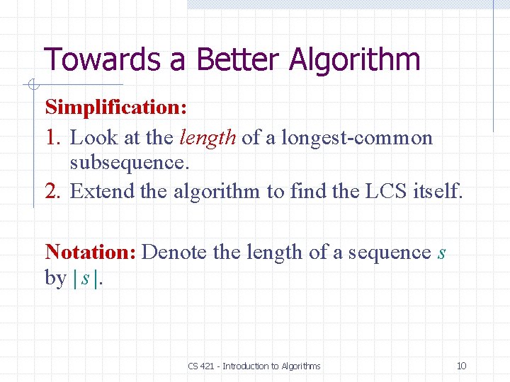
Towards a Better Algorithm Simplification: 1. Look at the length of a longest-common subsequence. 2. Extend the algorithm to find the LCS itself. Notation: Denote the length of a sequence s by | s |. CS 421 - Introduction to Algorithms 10

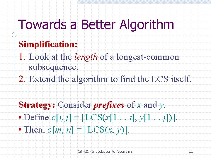
Towards a Better Algorithm Simplification: 1. Look at the length of a longest-common subsequence. 2. Extend the algorithm to find the LCS itself. Strategy: Consider prefixes of x and y. • Define c[i, j] = | LCS(x[1. . i], y[1. . j]) |. • Then, c[m, n] = | LCS(x, y) |. CS 421 - Introduction to Algorithms 11

Recursive Formulation Theorem. c[i, j] = c[i– 1, j– 1] + 1 if x[i] = y[j], max{c[i– 1, j], c[i, j– 1]} otherwise. CS 421 - Introduction to Algorithms 12

Recursive Formulation Theorem. c[i– 1, j– 1] + 1 if x[i] = y[j], max{c[i– 1, j], c[i, j– 1]} otherwise. c[i, j] = Proof. Case x[i] = y[ j]: 1 2 m L x: y: i 1 2 = j CS 421 - Introduction to Algorithms L n 13

Recursive Formulation Theorem. c[i– 1, j– 1] + 1 if x[i] = y[j], max{c[i– 1, j], c[i, j– 1]} otherwise. c[i, j] = Proof. Case x[i] = y[ j]: 1 2 m L x: y: i 1 2 = j L n Let z[1. . k] = LCS(x[1. . i], y[1. . j]), where c[i, j] = k. Then, z[k] = x[i], or else z could be extended. Thus, z[1. . k– 1] 14 is CS of x[1. . i– 1] and y[1. . j– 1].

Proof (cont'd) Claim: z[1. . k– 1] = LCS(x[1. . i– 1], y[1. . j– 1]). Suppose w is a longer CS of x[1. . i– 1] and y[1. . j– 1], that is, | w | > k– 1. Then, cut and paste: w || z[k] (w concatenated with z[k]) is a common subsequence of x[1. . i] and y[1. . j] with | w || z[k] | > k. Contradiction, proving the claim. CS 421 - Introduction to Algorithms 15

Proof (cont'd) Claim: z[1. . k– 1] = LCS(x[1. . i– 1], y[1. . j– 1]). Suppose w is a longer CS of x[1. . i– 1] and y[1. . j– 1], that is, | w | > k– 1. Then, cut and paste: w || z[k] (w concatenated with z[k]) is a common subsequence of x[1. . i] and y[1. . j] with | w || z[k] | > k. Contradiction, proving the claim. Thus, c[i– 1, j– 1] = k– 1, which implies that c[i, j] = c[i– 1, j– 1] + 1. Other cases are similar. CS 421 - Introduction to Algorithms 16

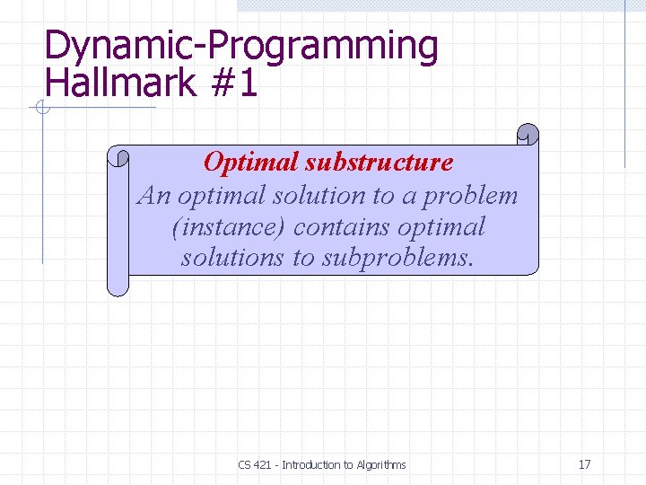
Dynamic-Programming Hallmark #1 Optimal substructure An optimal solution to a problem (instance) contains optimal solutions to subproblems. CS 421 - Introduction to Algorithms 17

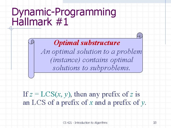
Dynamic-Programming Hallmark #1 Optimal substructure An optimal solution to a problem (instance) contains optimal solutions to subproblems. If z = LCS(x, y), then any prefix of z is an LCS of a prefix of x and a prefix of y. CS 421 - Introduction to Algorithms 18

Recursive Algorithm for LCS(x, y, i, j) if x[i] = y[ j] then c[i, j] LCS(x, y, i– 1, j– 1) + 1 else c[i, j] max{ LCS(x, y, i– 1, j), LCS(x, y, i, j– 1)} CS 421 - Introduction to Algorithms 19

Recursive Algorithm for LCS(x, y, i, j) if x[i] = y[ j] then c[i, j] LCS(x, y, i– 1, j– 1) + 1 else c[i, j] max{ LCS(x, y, i– 1, j), LCS(x, y, i, j– 1)} Worst-case: x[i] y[ j], in which case the algorithm evaluates two sub-problems, each with only one parameter decremented. CS 421 - Introduction to Algorithms 20

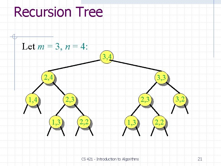
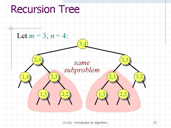
Recursion Tree Let m = 3, n = 4: 3, 4 2, 4 3, 3 2, 3 1, 4 1, 3 3, 2 2, 3 2, 2 1, 3 CS 421 - Introduction to Algorithms 2, 2 21

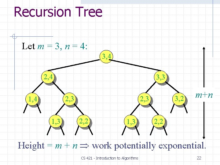
Recursion Tree Let m = 3, n = 4: 3, 4 2, 4 3, 3 2, 3 1, 4 1, 3 3, 2 2, 3 2, 2 1, 3 m+n 2, 2 Height = m + n work potentially exponential. CS 421 - Introduction to Algorithms 22

Recursion Tree Let m = 3, n = 4: 3, 4 2, 3 1, 4 1, 3 same subproblem 2, 2 1, 3 CS 421 - Introduction to Algorithms 3, 3 3, 2 2, 3 2, 2 23

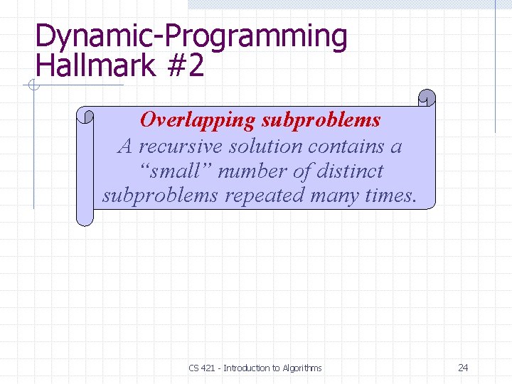
Dynamic-Programming Hallmark #2 Overlapping subproblems A recursive solution contains a “small” number of distinct subproblems repeated many times. CS 421 - Introduction to Algorithms 24

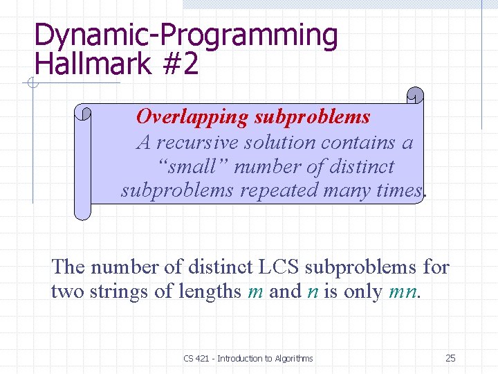
Dynamic-Programming Hallmark #2 Overlapping subproblems A recursive solution contains a “small” number of distinct subproblems repeated many times. The number of distinct LCS subproblems for two strings of lengths m and n is only mn. CS 421 - Introduction to Algorithms 25

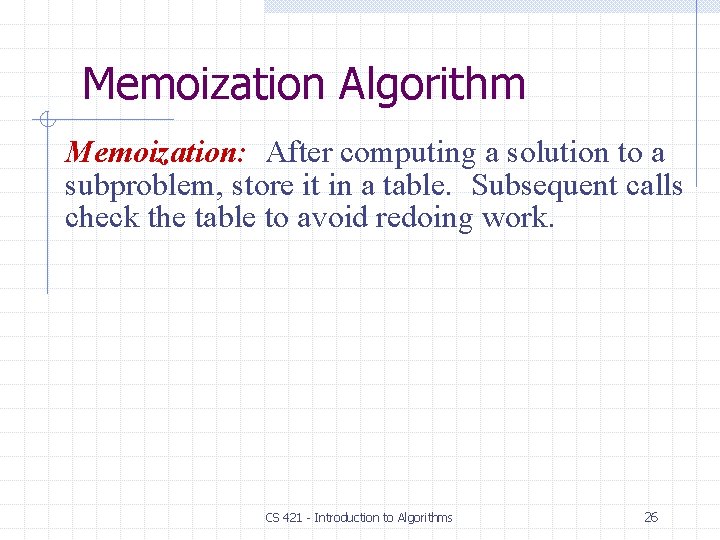
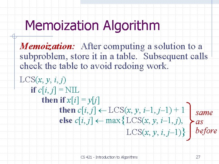
Memoization Algorithm Memoization: After computing a solution to a subproblem, store it in a table. Subsequent calls check the table to avoid redoing work. CS 421 - Introduction to Algorithms 26

Memoization Algorithm Memoization: After computing a solution to a subproblem, store it in a table. Subsequent calls check the table to avoid redoing work. LCS(x, y, i, j) if c[i, j] = NIL then if x[i] = y[j] then c[i, j] LCS(x, y, i– 1, j– 1) + 1 else c[i, j] max{ LCS(x, y, i– 1, j), LCS(x, y, i, j– 1)} CS 421 - Introduction to Algorithms same as before 27

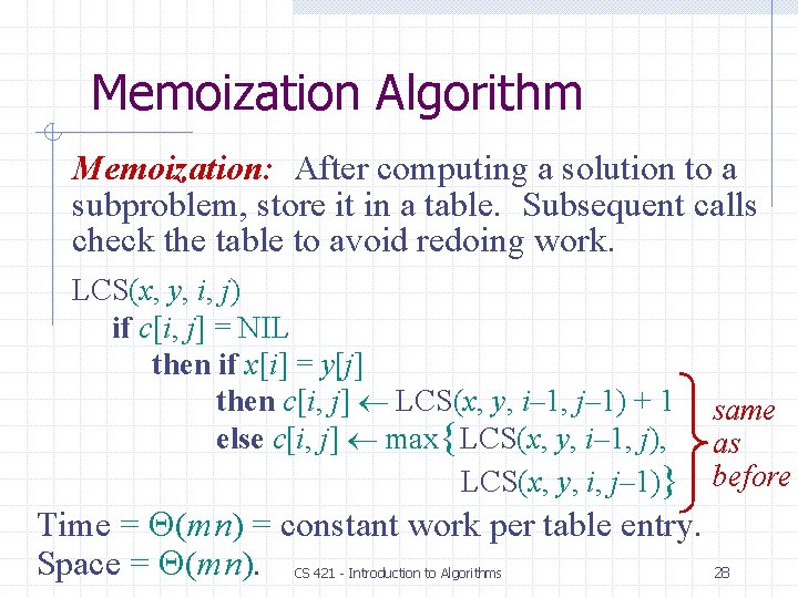
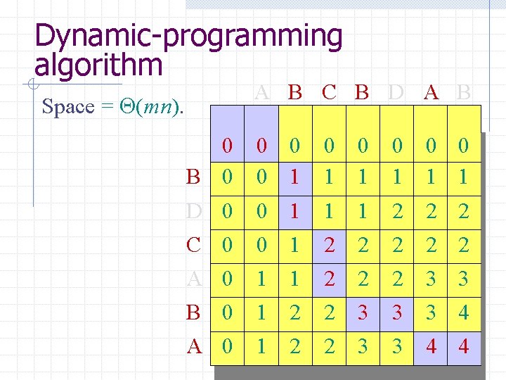
Memoization Algorithm Memoization: After computing a solution to a subproblem, store it in a table. Subsequent calls check the table to avoid redoing work. LCS(x, y, i, j) if c[i, j] = NIL then if x[i] = y[j] then c[i, j] LCS(x, y, i– 1, j– 1) + 1 else c[i, j] max{ LCS(x, y, i– 1, j), LCS(x, y, i, j– 1)} same as before Time = (mn) = constant work per table entry. Space = (mn). 28 CS 421 - Introduction to Algorithms

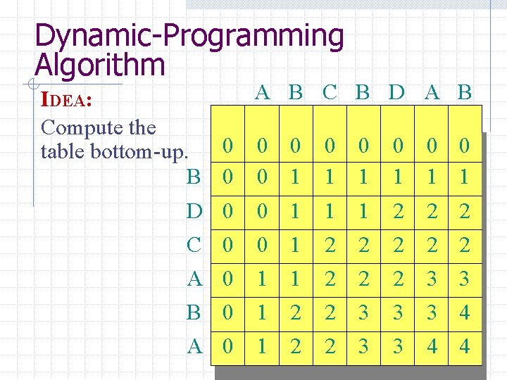
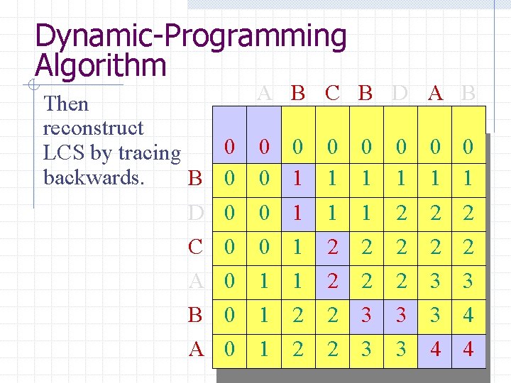
Dynamic-Programming Algorithm IDEA: Compute the table bottom-up. B D C A B A A B C B D A B 0 0 0 0 0 0 1 1 1 0 0 1 1 1 1 2 2 2 2 3 3 0 0 1 1 2 2 2 3 3 0 0 1 1 2 2 3 3 4 4

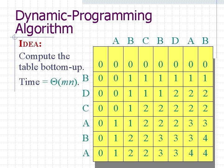
Dynamic-Programming Algorithm IDEA: Compute the table bottom-up. Time = (mn). B D C A B A A B C B D A B 0 0 0 0 0 0 1 1 1 0 0 1 1 1 1 2 2 2 2 3 3 0 0 1 1 2 2 2 3 3 0 0 1 1 2 2 3 3 4 4

Dynamic-Programming Algorithm Then 00 reconstruct 0 LCS by tracing 0 backwards. B 0 0 D 0 0 C 0 0 A 0 0 B 0 0 A 00 0 0 0 1 1 1 B C B D A B 0 01 1 1 2 2 0 0 1 1 22 2 2 2 0 0 1 1 2 2 2 2 33 3 3 3 0 0 1 1 2 2 2 2 3 3 44 4 0 0 1 1 2 2 3 3 4 4 44 4

Dynamic-programming algorithm Space = (mn). B D C A B A 00 0 0 0 A 00 0 0 0 1 1 1 B C B D A B 0 01 1 1 2 2 0 0 1 1 22 2 2 2 0 0 1 1 2 2 2 2 33 3 3 3 0 0 1 1 2 2 2 2 3 3 44 4 0 0 1 1 2 2 3 3 4 4 44 4