Introduction to Algorithms Chapter 3 Growth of Functions

Introduction to Algorithms Chapter 3: Growth of Functions

How fast will your program run? n The running time of your program will depend upon: q q q n The algorithm The input Your implementation of the algorithm in a programming language The compiler you use The OS on your computer Your computer hardware Our Motivation: analyze the running time of an algorithm as a function of only simple parameters of the input. 2

Complexity n Complexity is the number of steps required to solve a problem. n The goal is to find the best algorithm to solve the problem with a less number of steps n Complexity of Algorithms q q The size of the problem is a measure of the quantity of the input data n The time needed by an algorithm, expressed as a function of the size of the problem (it solves), is called the (time) complexity of the algorithm T(n) 3

Basic idea: counting operations n Running Time: Number of primitive steps that are executed q most statements roughly require the same amount of time n n y=m*x+b c = 5 / 9 * (t - 32 ) z = f(x) + g(y) Each algorithm performs a sequence of basic operations: q q q Arithmetic: Comparison: Assignment: Branching: … (low + high)/2 if ( x > 0 ) … temp = x while ( true ) { … } 4

Basic idea: counting operations n Idea: count the number of basic operations performed on the input. n Difficulties: q q q Which operations are basic? Not all operations take the same amount of time. Operations take different times with different hardware or compilers 5

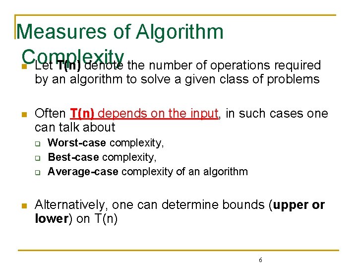
Measures of Algorithm Complexity n Let T(n) denote the number of operations required by an algorithm to solve a given class of problems n Often T(n) depends on the input, in such cases one can talk about q q q n Worst-case complexity, Best-case complexity, Average-case complexity of an algorithm Alternatively, one can determine bounds (upper or lower) on T(n) 6

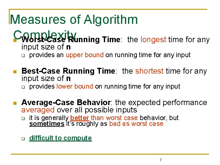
Measures of Algorithm Complexity n Worst-Case Running Time: the longest time for any input size of n q n Best-Case Running Time: the shortest time for any input size of n q n provides an upper bound on running time for any input provides lower bound on running time for any input Average-Case Behavior: the expected performance averaged over all possible inputs q it is generally better than worst case behavior, but sometimes it’s roughly as bad as worst case q difficult to compute 7

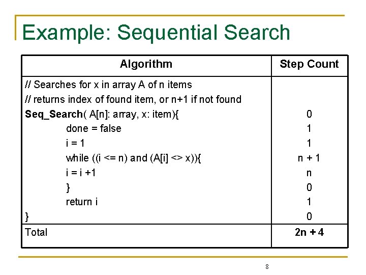
Example: Sequential Search Algorithm Step Count // Searches for x in array A of n items // returns index of found item, or n+1 if not found Seq_Search( A[n]: array, x: item){ done = false i=1 while ((i <= n) and (A[i] <> x)){ i = i +1 } return i } 0 1 1 n+1 n 0 1 0 Total 2 n + 4 8

Example: Sequential Search n worst-case running time q q q n when x is not in the original array A in this case, while loop needs 2(n + 1) comparisons + c other operations So, T(n) = 2 n + 2 + c Linear complexity best-case running time q q q when x is found in A[1] in this case, while loop needs 2 comparisons + c other operations So, T(n) = 2 + c Constant complexity 9

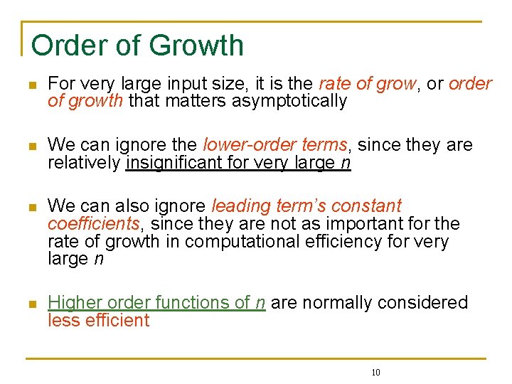
Order of Growth n For very large input size, it is the rate of grow, or order of growth that matters asymptotically n We can ignore the lower-order terms, since they are relatively insignificant for very large n n We can also ignore leading term’s constant coefficients, since they are not as important for the rate of growth in computational efficiency for very large n n Higher order functions of n are normally considered less efficient 10

Asymptotic Notation n , O, , o, w n Used to describe the running times of algorithms n Instead of exact running time, say (n 2) n Defined for functions whose domain is the set of natural numbers, N n Determine sets of functions, in practice used to compare two functions 11

Asymptotic Notation n By now you should have an intuitive feel for asymptotic (big-O) notation: q n What does O(n) running time mean? O(n 2)? O(n lg n)? Our first task is to define this notation more formally and completely 12

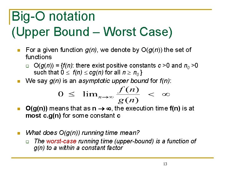
Big-O notation (Upper Bound – Worst Case) n n For a given function g(n), we denote by O(g(n)) the set of functions q O(g(n)) = {f(n): there exist positive constants c >0 and n 0 >0 such that 0 f(n) cg(n) for all n n 0 } We say g(n) is an asymptotic upper bound for f(n): O(g(n)) means that as n , the execution time f(n) is at most c. g(n) for some constant c What does O(g(n)) running time mean? q The worst-case running time (upper-bound) is a function of g(n) to a within a constant factor 13

Big-O notation (Upper Bound – Worst Case) c. g(n) time f(n) n 0 n f(n) = O(g(n)) 14

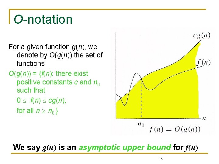
O-notation For a given function g(n), we denote by O(g(n)) the set of functions O(g(n)) = {f(n): there exist positive constants c and n 0 such that 0 f(n) cg(n), for all n n 0 } We say g(n) is an asymptotic upper bound for f(n) 15

Big-O notation (Upper Bound – Worst Case) n n This is a mathematically formal way of ignoring constant factors, and looking only at the “shape” of the function f(n)=O(g(n)) should be considered as saying that “f(n) is at most g(n), up to constant factors”. We usually will have f(n) be the running time of an algorithm and g(n) a nicely written function E. g. The running time of insertion sort algorithm is O(n 2) Example: 2 n 2 = O(n 3), with c = 1 and n 0 = 2. New n 16

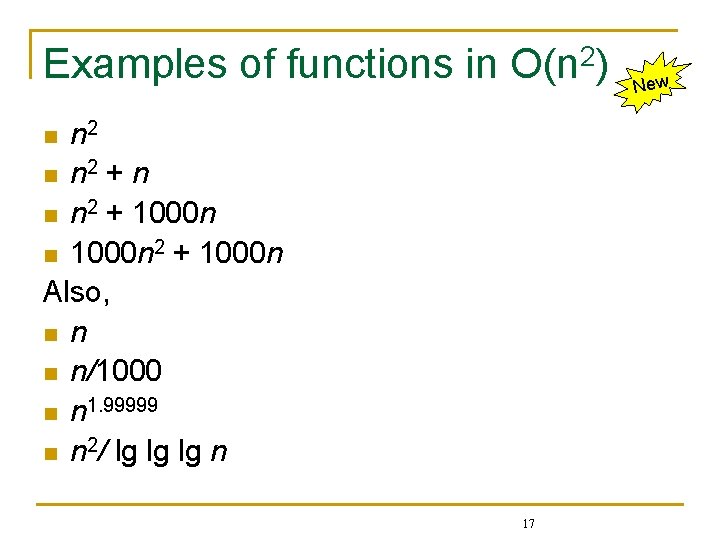
Examples of functions in O(n 2) n 2 n n 2 + n n n 2 + 1000 n n 1000 n 2 + 1000 n Also, n n/1000 n n 1. 99999 n n 2/ lg lg lg n n 17 New

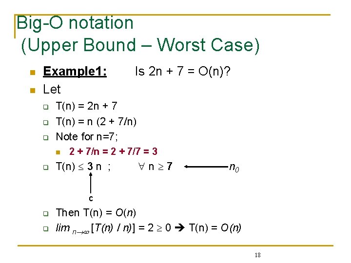
Big-O notation (Upper Bound – Worst Case) n n Example 1: Let q q q T(n) = 2 n + 7 T(n) = n (2 + 7/n) Note for n=7; n q Is 2 n + 7 = O(n)? 2 + 7/n = 2 + 7/7 = 3 T(n) 3 n ; n 7 n 0 c q q Then T(n) = O(n) lim n [T(n) / n)] = 2 0 T(n) = O(n) 18

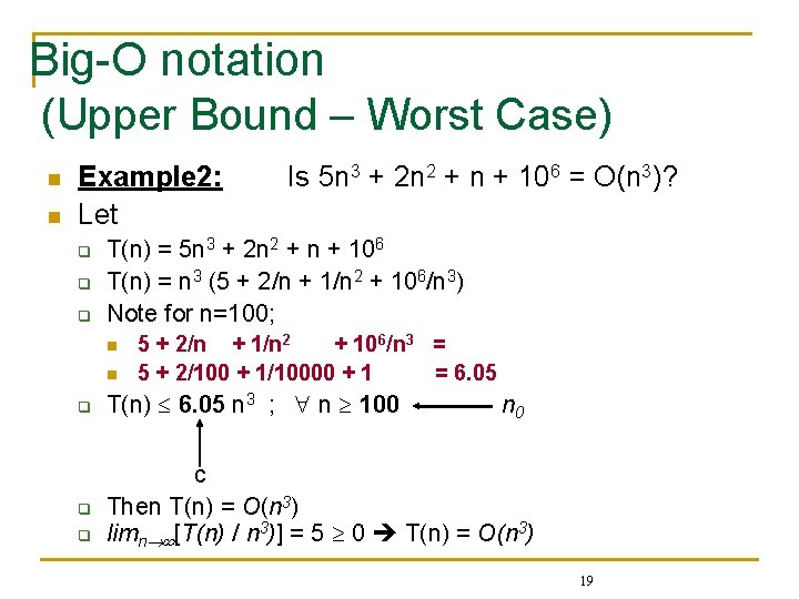
Big-O notation (Upper Bound – Worst Case) n n Example 2: Let q q q Is 5 n 3 + 2 n 2 + n + 106 = O(n 3)? T(n) = 5 n 3 + 2 n 2 + n + 106 T(n) = n 3 (5 + 2/n + 1/n 2 + 106/n 3) Note for n=100; n n 5 + 2/n + 1/n 2 + 106/n 3 = 5 + 2/100 + 1/10000 + 1 = 6. 05 q T(n) 6. 05 n 3 ; n 100 q c Then T(n) = O(n 3) limn [T(n) / n 3)] = 5 0 T(n) = O(n 3) q n 0 19

Big-O notation (Upper Bound – Worst Case) n n Express the execution time as a function of the input size n Since only the growth rate matters, we can ignore the multiplicative constants and the lower order terms, e. g. , q n, n+1, n+80, 40 n, n+log n is O(n) q n 1. 1 + 100000 n is O(n 1. 1) q n 2 is O(n 2) q 3 n 2 + 6 n + log n + 24. 5 is O(n 2) n O(1) < O(log n) < O((log n)3) < O(n 2) < O(n 3) < O(nlog n) < O(2 sqrt(n)) < O(2 n) < O(n!) < O(nn) n Constant < Logarithmic < Linear < Quadratic< Cubic < Polynomial < Factorial < Exponential 20

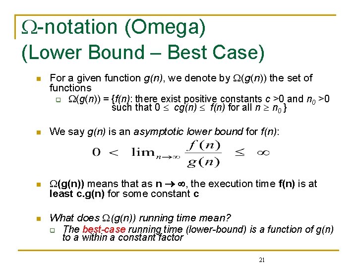
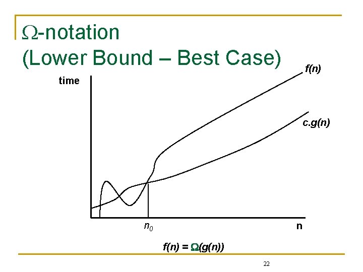
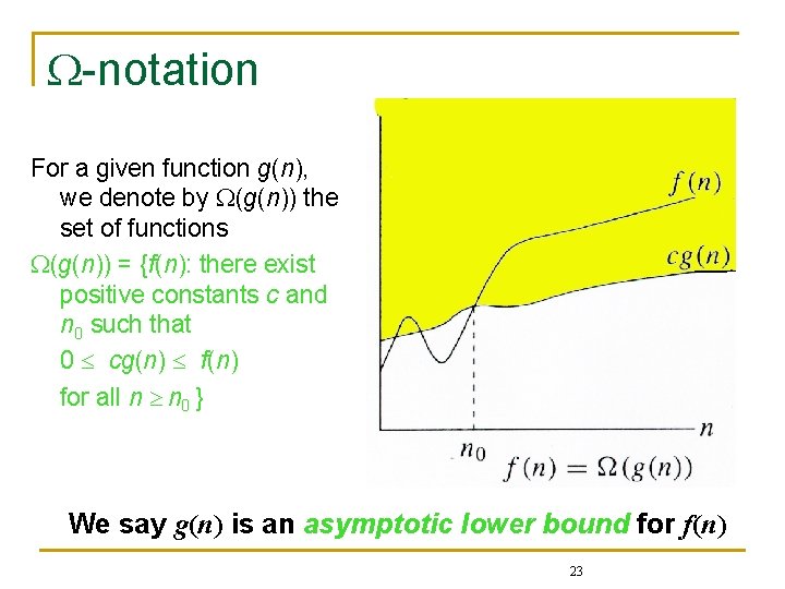
-notation (Omega) (Lower Bound – Best Case) n For a given function g(n), we denote by (g(n)) the set of functions q (g(n)) = {f(n): there exist positive constants c >0 and n 0 >0 such that 0 cg(n) f(n) for all n n 0 } n We say g(n) is an asymptotic lower bound for f(n): n (g(n)) means that as n , the execution time f(n) is at least c. g(n) for some constant c n What does (g(n)) running time mean? q The best-case running time (lower-bound) is a function of g(n) to a within a constant factor 21

-notation (Lower Bound – Best Case) f(n) time c. g(n) n 0 n f(n) = (g(n)) 22

-notation For a given function g(n), we denote by (g(n)) the set of functions (g(n)) = {f(n): there exist positive constants c and n 0 such that 0 cg(n) f(n) for all n n 0 } We say g(n) is an asymptotic lower bound for f(n) 23

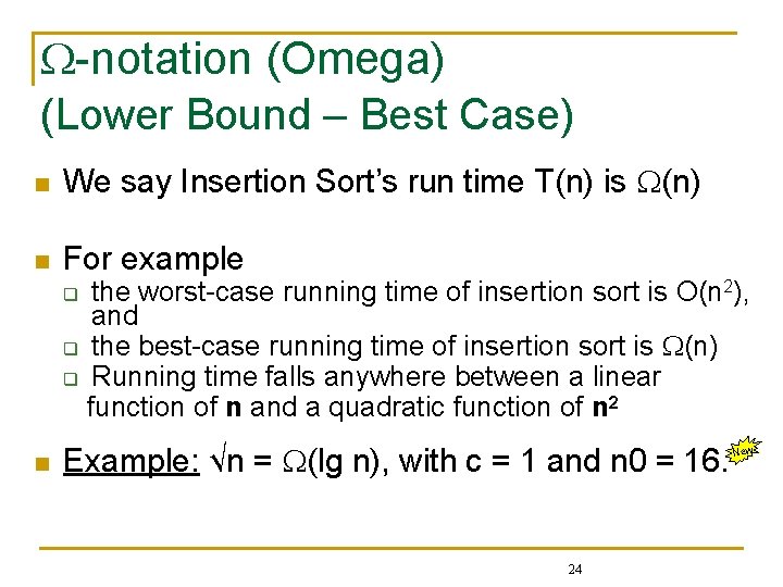
-notation (Omega) (Lower Bound – Best Case) n We say Insertion Sort’s run time T(n) is (n) n For example the worst-case running time of insertion sort is O(n 2), and q the best-case running time of insertion sort is (n) q Running time falls anywhere between a linear function of n and a quadratic function of n 2 q n Example: √n = (lg n), with c = 1 and n 0 = 16. 24 New

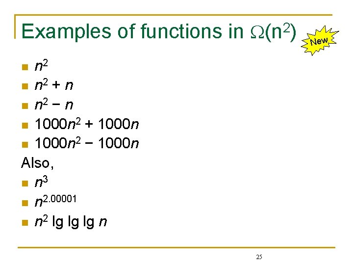
Examples of functions in (n 2) n 2 n n 2 + n n n 2 − n n 1000 n 2 + 1000 n n 1000 n 2 − 1000 n Also, n n 3 n n 2. 00001 n n 2 lg lg lg n n 25 New

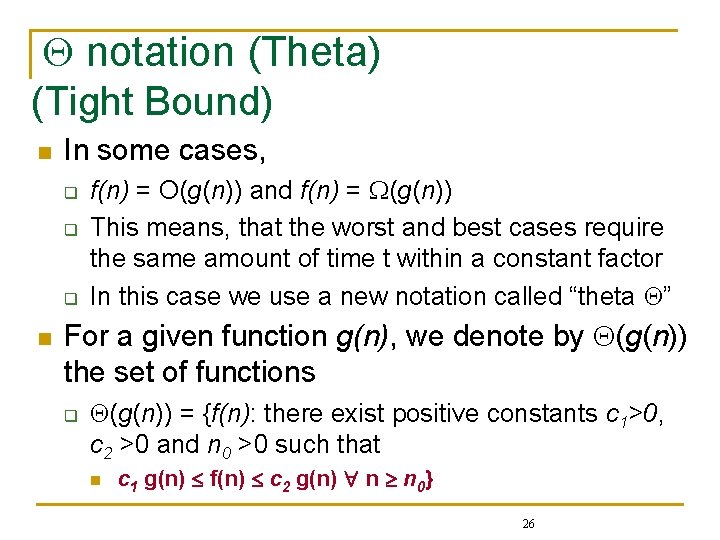
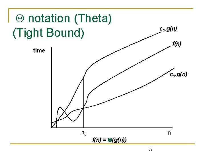
notation (Theta) (Tight Bound) n In some cases, q q q n f(n) = O(g(n)) and f(n) = (g(n)) This means, that the worst and best cases require the same amount of time t within a constant factor In this case we use a new notation called “theta ” For a given function g(n), we denote by (g(n)) the set of functions q (g(n)) = {f(n): there exist positive constants c 1>0, c 2 >0 and n 0 >0 such that n c 1 g(n) f(n) c 2 g(n) n n 0} 26

notation (Theta) (Tight Bound) n We say g(n) is an asymptotic tight bound for f(n): n Theta notation q n (g(n)) means that as n , the execution time f(n) is at most c 2. g(n) and at least c 1. g(n) for some constants c 1 and c 2. f(n) = (g(n)) if and only if q f(n) = O(g(n)) & f(n) = (g(n)) 27

notation (Theta) (Tight Bound) c 2. g(n) f(n) time c 1. g(n) n 0 n f(n) = (g(n)) 28

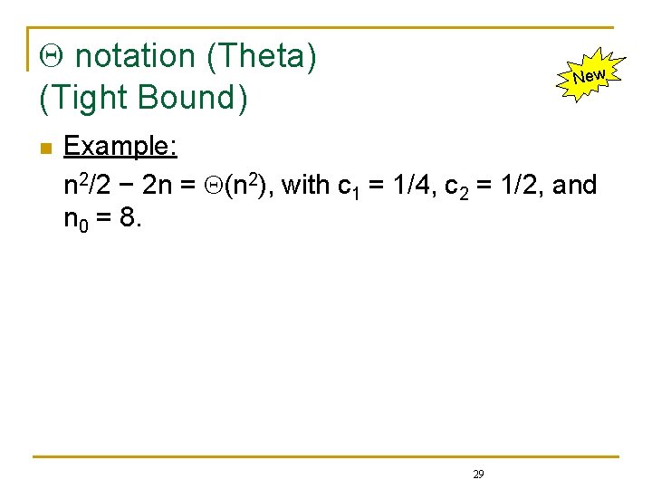
notation (Theta) (Tight Bound) n New Example: n 2/2 − 2 n = (n 2), with c 1 = 1/4, c 2 = 1/2, and n 0 = 8. 29