Introduction to Algorithmic Trading Strategies Lecture 8 Risk

Introduction to Algorithmic Trading Strategies Lecture 8 Risk Management Haksun Li haksun. li@numericalmethod. com www. numericalmethod. com

Outline � Value at Risk (Va. R) � Extreme Value Theory (EVT)

References � AJ Mc. Neil. Extreme Value Theory for Risk Managers. 1999. � Blake Le. Baron, Ritirupa Samanta. Extreme Value Theory and Fat Tails in Equity Markets. November 2005.

Risks � Financial theories say: � the most important single source of profit is risk. � profit ∝ risk. �I personally do not agree.

What Are Some Risks? (1) � Bonds: � duration (sensitivity to interest rate) � convexity � term structure models � Credit: � rating � default models

What Are Some Risks? (2) � Stocks � volatility � correlations � beta � Derivatives � delta � gamma � vega

What Are Some Risks? (3) � FX � volatility � target zones � spreads � term structure models of related currencies

Other Risks? � Too many to enumerate… � natural disasters, e. g. , earthquake � war � politics � operational risk � regulatory risk � wide spread rumors � alien attack!!! � Practically infinitely many of them…

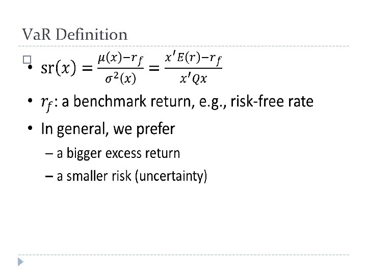
Va. R Definition �

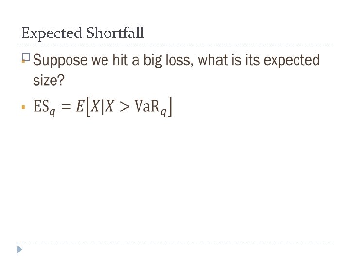
Expected Shortfall �

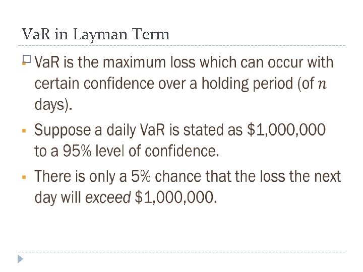
Va. R in Layman Term �

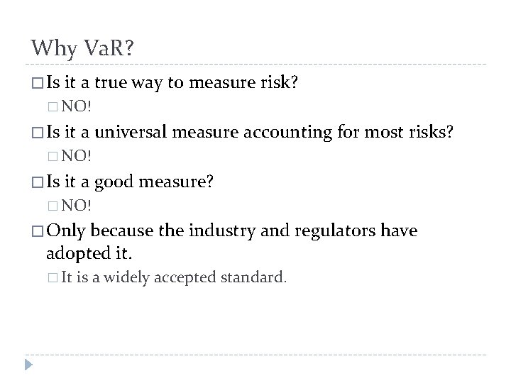
Why Va. R? � Is it a true way to measure risk? � NO! � Is it a universal measure accounting for most risks? � NO! � Is it a good measure? � NO! � Only because the industry and regulators have adopted it. � It is a widely accepted standard.

Va. R Computations � Historical Simulation � Variance-Co. Variance � Monte Carlo simulation

Historical Simulations � Take a historical returns time series as the returns distribution. � Compute the loss distribution from the historical returns distribution.

Historical Simulations Advantages � Simplest � Non-parametric, no assumption of distributions, no possibility of estimation error

Historical Simulations Dis-Advantages � As all historical returns carry equal weights, it runs the risk of over-/under- estimate the recent trends. � Sample period may not be representative of the risks. � History may not repeat itself. � Cannot accommodate for new risks. � Cannot incorporate subjective information.

Variance-Co. Variance �

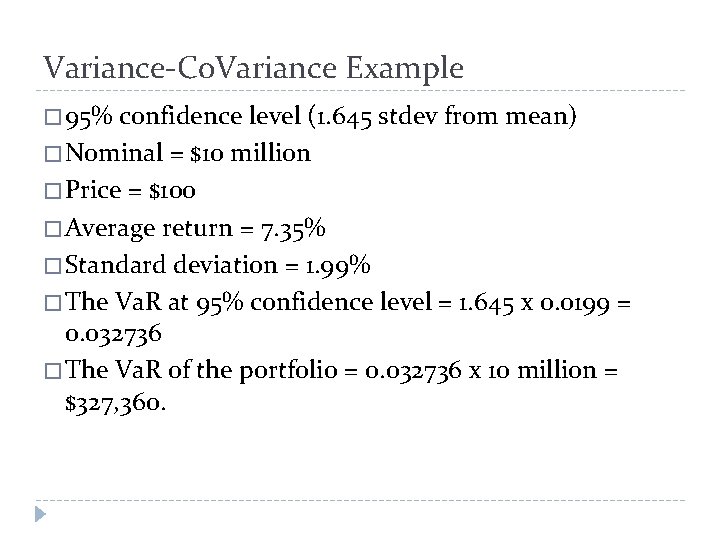
Variance-Co. Variance Example � 95% confidence level (1. 645 stdev from mean) � Nominal = $10 million � Price = $100 � Average return = 7. 35% � Standard deviation = 1. 99% � The Va. R at 95% confidence level = 1. 645 x 0. 0199 = 0. 032736 � The Va. R of the portfolio = 0. 032736 x 10 million = $327, 360.

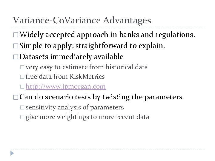
Variance-Co. Variance Advantages � Widely accepted approach in banks and regulations. � Simple to apply; straightforward to explain. � Datasets immediately available � very easy to estimate from historical data � free data from Risk. Metrics � http: //www. jpmorgan. com � Can do scenario tests by twisting the parameters. � sensitivity analysis of parameters � give more weightings to more recent data

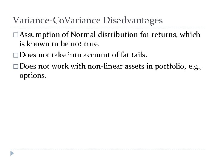
Variance-Co. Variance Disadvantages � Assumption of Normal distribution for returns, which is known to be not true. � Does not take into account of fat tails. � Does not work with non-linear assets in portfolio, e. g. , options.

Monte Carlo Simulation � You create your own returns distributions. � historical data � implied data � economic scenarios � Simulate the joint distributions many times. � Compute the empirical returns distribution of the portfolio. � Compute the (e. g. , 1%, 5%) quantile.

Monte Carlo Simulation Advantages � Does not assume any specific models, or forms of distributions. � Can incorporate any information, even subjective views. � Can do scenario tests by twisting the parameters. � sensitivity analysis of parameters � give more weightings to more recent data � Can work with non-linear assets, e. g. , options. � Can track path-dependence.

Monte Carlo Simulation Disadvantages � Slow. � To increase the precision by a factor of 10, we must make 100 times more simulations. � Various variance reduction techniques apply. � antithetic variates � control variates � importance sampling � stratified sampling � Difficult to build a (high) multi-dimensional joint distribution from data.

100 -Year Market Crash � How do we incorporate rare events into our returns distributions, hence enhanced risk management? � Statistics works very well when you have a large amount of data. � How do we analyze for (very) small samples?

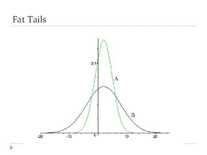
Fat Tails

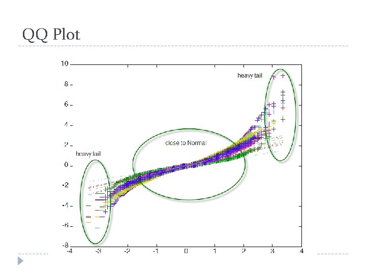
QQ � A QQ plots display the quintiles of the sample data against those of a standard normal distribution. � This is the first diagnostic tool in determining whether the data have fat tails.

QQ Plot

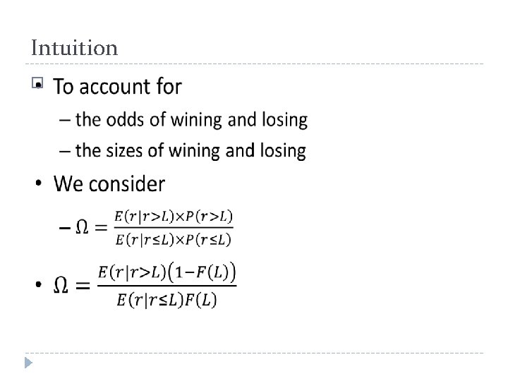
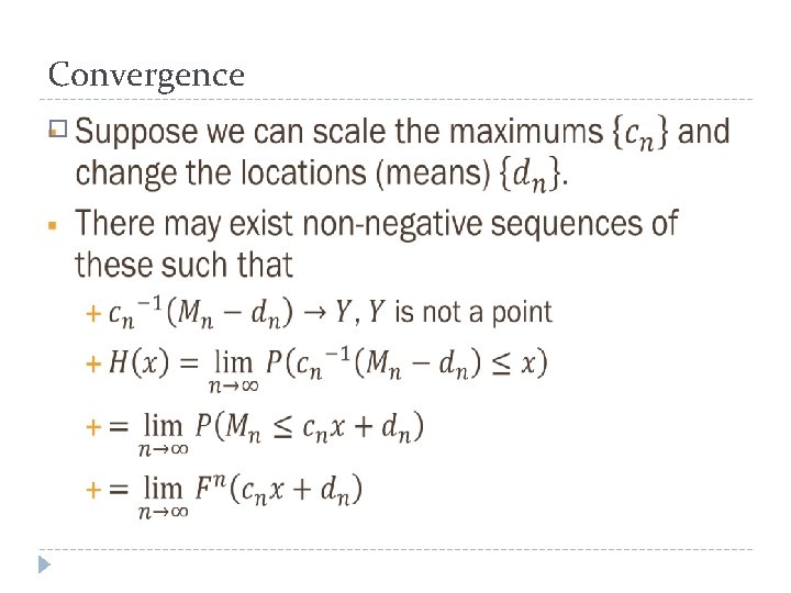
Asymptotic Properties � The (normalized) mean of a the sample mean of a large population is normally distributed, regardless of the generating distribution. � What about the sample maximum?

Intuition �

Convergence �

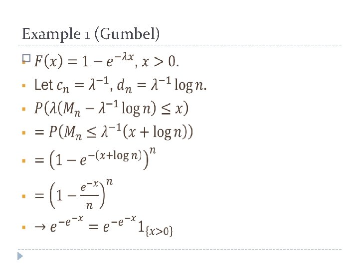
Example 1 (Gumbel) �

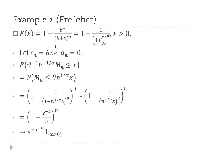
Example 2 (Fre´chet) �

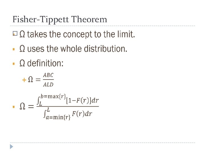
Fisher-Tippett Theorem �

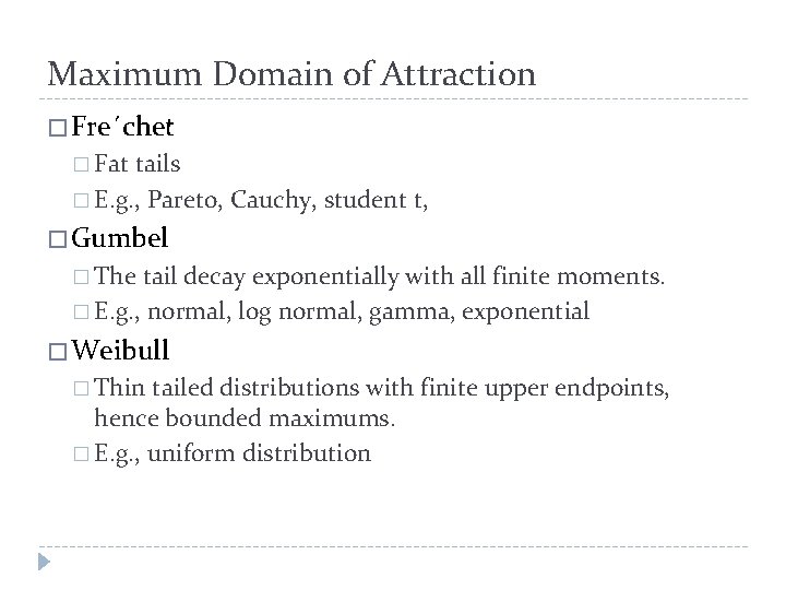
Maximum Domain of Attraction � Fre´chet � Fat tails � E. g. , Pareto, Cauchy, student t, � Gumbel � The tail decay exponentially with all finite moments. � E. g. , normal, log normal, gamma, exponential � Weibull � Thin tailed distributions with finite upper endpoints, hence bounded maximums. � E. g. , uniform distribution

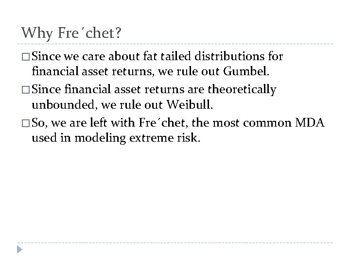
Why Fre´chet? � Since we care about fat tailed distributions for financial asset returns, we rule out Gumbel. � Since financial asset returns are theoretically unbounded, we rule out Weibull. � So, we are left with Fre´chet, the most common MDA used in modeling extreme risk.

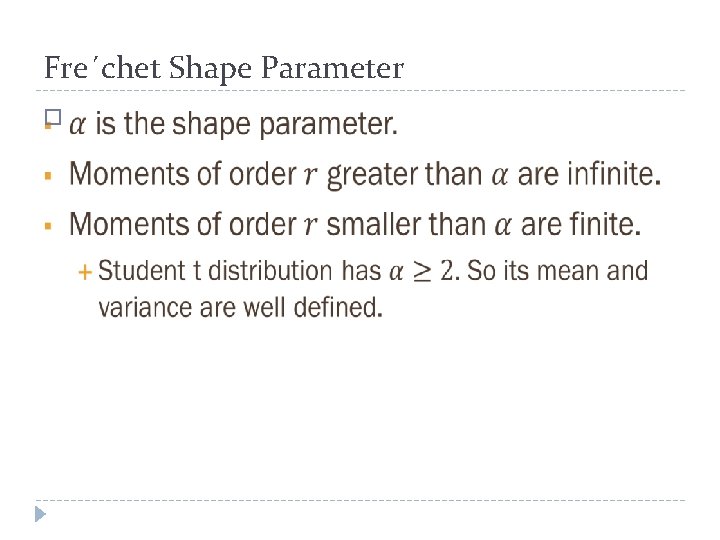
Fre´chet Shape Parameter �

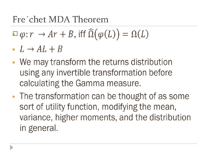
Fre´chet MDA Theorem �

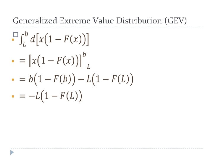
Generalized Extreme Value Distribution (GEV) �

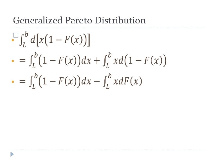
Generalized Pareto Distribution �

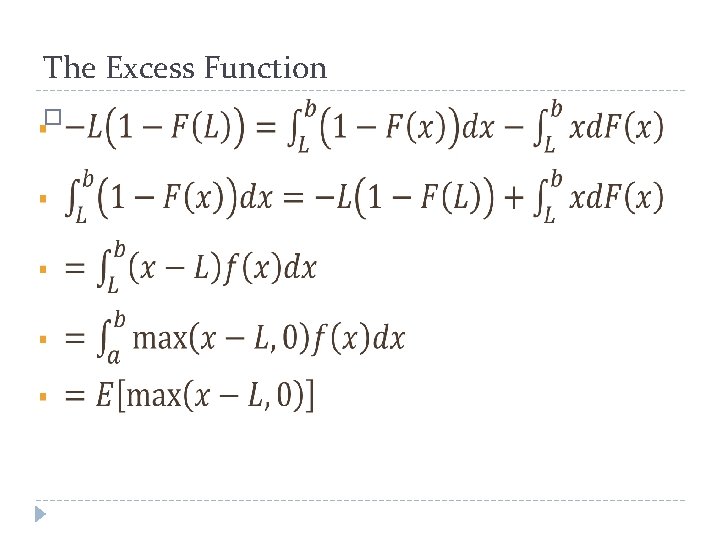
The Excess Function �

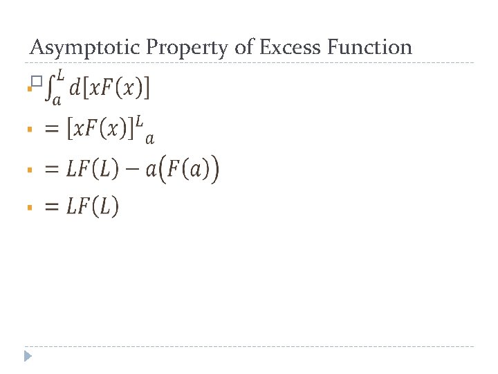
Asymptotic Property of Excess Function �

Tail Index Estimation by Quantiles � Hill, 1975 � Pickands, 1975 � Dekkers and De. Haan, 1990

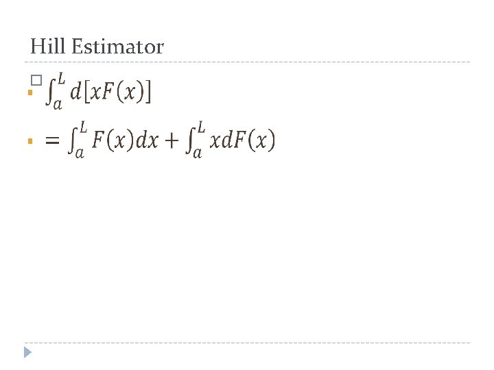
Hill Estimator �

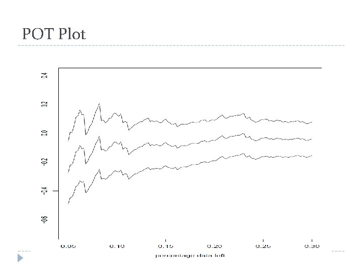
POT Plot

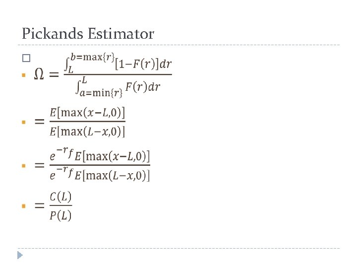
Pickands Estimator �

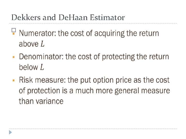
Dekkers and De. Haan Estimator �

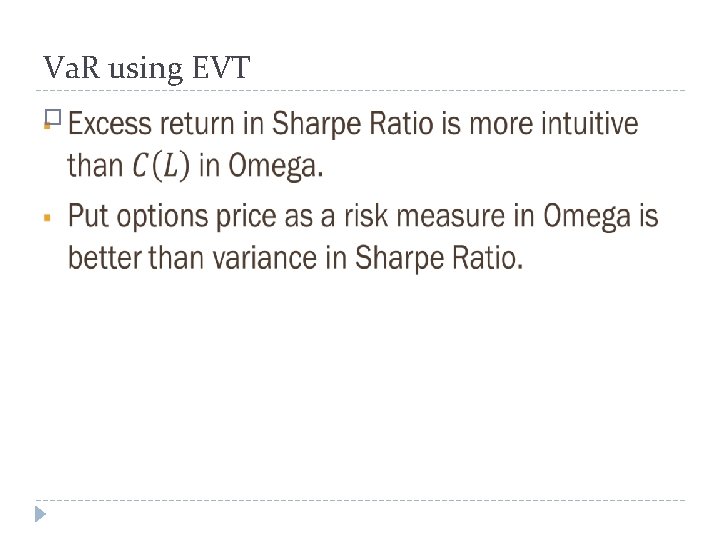
Va. R using EVT �

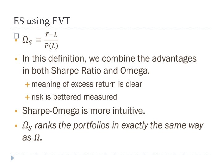
ES using EVT �

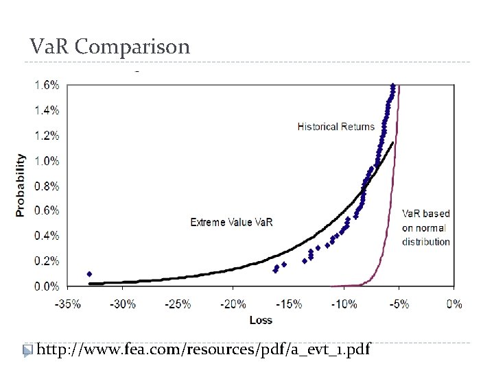
Va. R Comparison � http: //www. fea. com/resources/pdf/a_evt_1. pdf