Introduction to Adjoint Methods in Meteorology Rolf Langland

Introduction to Adjoint Methods in Meteorology Rolf Langland Data Assimilation Section Naval Research Laboratory Monterey, CA langland@nrlmry. navy. mil Including Material Provided by Dr. Ronald M. Errico (NASA-UMBC) JCSDA Summer Colloquium on Data Assimilation Santa Fe, N. M. , 31 July 2012 1

Adjoint Methods Introduction 1. What is an adjoint model 2. Examples of adjoint equations 3. Interpretation of adjoint sensitivity 4. Development / testing of adjoint code 5. Misunderstandings about adjoint methods Please ask questions during presentation if something is not clear! 2

What is an Adjoint Model? [NWP context] • The transpose of a tangent linear version of a forecast model • It can be used to estimate the sensitivity of a forecast aspect (J) with respect to model initial conditions and parameters • Sensitivity information is useful for short-range forecasts (72 hr or less), subject to tangentlinear approximations 3

Why use adjoint models ? • Require information about sensitivity to initial conditions, but cannot construct the inverse of a numerical forecast model … • An adjoint model can provide good estimates of initial condition sensitivity, consistent with actual dynamics of nonlinear forecast model (group velocity, etc. ) • Difficult or impossible to obtain this information by other methods 4

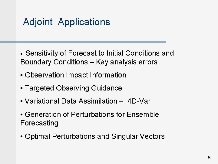
Adjoint Applications Sensitivity of Forecast to Initial Conditions and Boundary Conditions – Key analysis errors • • Observation Impact Information • Targeted Observing Guidance • Variational Data Assimilation – 4 D-Var • Generation of Perturbations for Ensemble Forecasting • Optimal Perturbations and Singular Vectors 5

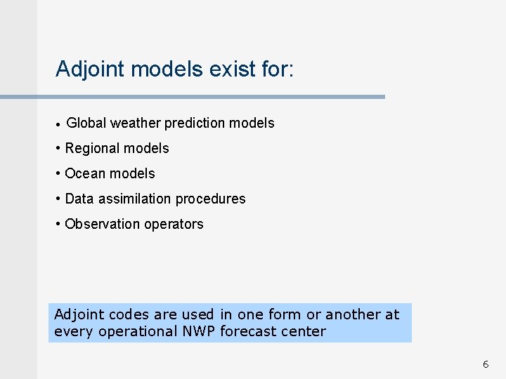
Adjoint models exist for: • Global weather prediction models • Regional models • Ocean models • Data assimilation procedures • Observation operators Adjoint codes are used in one form or another at every operational NWP forecast center 6

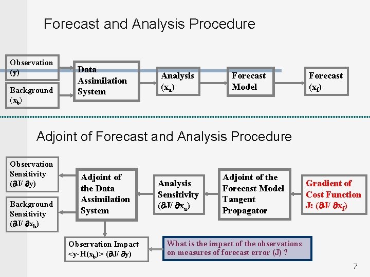
Forecast and Analysis Procedure Observation (y) Background (xb) Data Assimilation System Analysis (xa) Forecast Model Forecast (xf) Adjoint of Forecast and Analysis Procedure Observation Sensitivity ( J/ y) Background Sensitivity ( J/ xb) Adjoint of the Data Assimilation System Observation Impact <y-H(xb)> ( J/ y) Analysis Sensitivity ( J/ xa) Adjoint of the Forecast Model Tangent Propagator Gradient of Cost Function J: ( J/ xf) What is the impact of the observations on measures of forecast error (J) ? 7

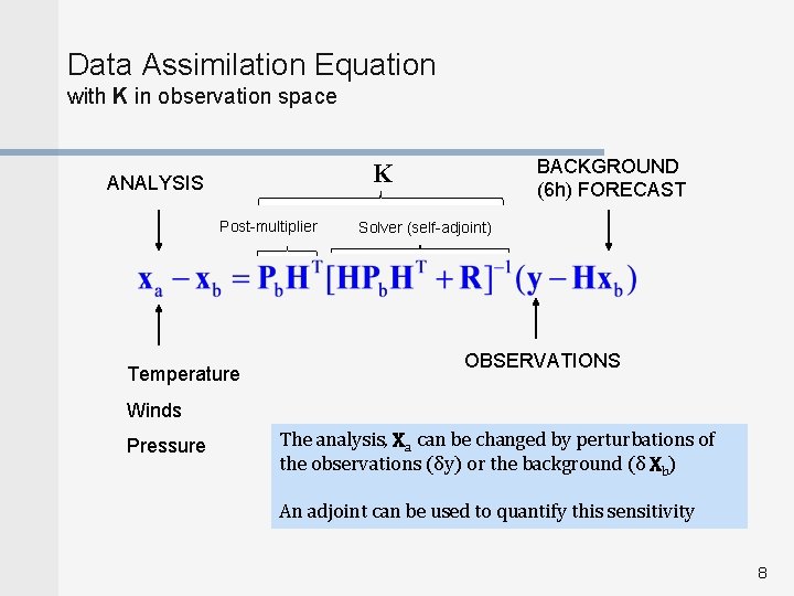
Data Assimilation Equation with K in observation space BACKGROUND (6 h) FORECAST K ANALYSIS Post-multiplier Temperature Solver (self-adjoint) OBSERVATIONS Winds Pressure The analysis, Xa can be changed by perturbations of the observations (δy) or the background (δ Xb) An adjoint can be used to quantify this sensitivity 8

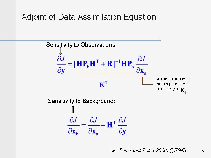
Adjoint of Data Assimilation Equation Sensitivity to Observations: Adjoint of forecast model produces sensitivity to Sensitivity to Background: see Baker and Daley 2000, QJRMS 9

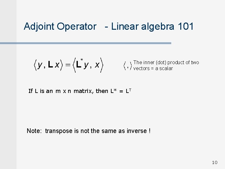
Adjoint Operator - Linear algebra 101 The inner (dot) product of two vectors = a scalar If L is an m x n matrix, then L* = LT Note: transpose is not the same as inverse ! 10

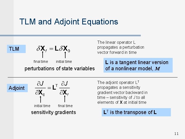
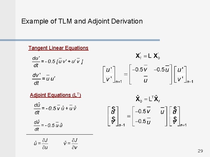
TLM and Adjoint Equations The linear operator L propagates a perturbation vector forward in time TLM final time initial time perturbations of state variables Adjoint initial time final time sensitivity gradients L is a tangent linear version of a nonlinear model, M The adjoint operator LT propagates a sensitivity gradient vector backward in time – sensitivity of J to all elements of X at initial time LT is the transpose of L 11

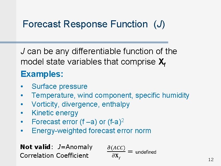
Forecast Response Function (J) J can be any differentiable function of the model state variables that comprise Xf Examples: • • • Surface pressure Temperature, wind component, specific humidity Vorticity, divergence, enthalpy Kinetic energy Forecast error (f –a) or (f-a)2 Energy-weighted forecast error norm Not valid: J=Anomaly Correlation Coefficient 12

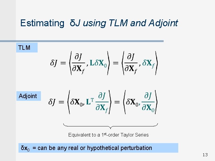
Estimating δJ using TLM and Adjoint TLM Adjoint Equivalent to a 1 st-order Taylor Series δx 0 = can be any real or hypothetical perturbation 13

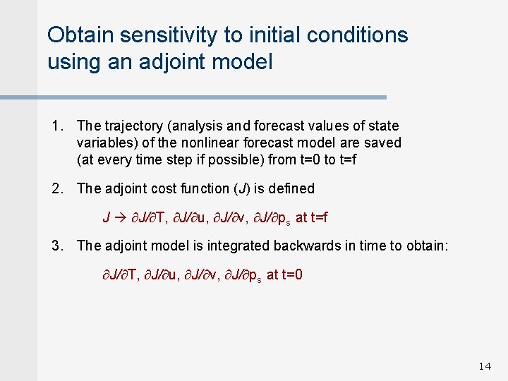
Obtain sensitivity to initial conditions using an adjoint model 1. The trajectory (analysis and forecast values of state variables) of the nonlinear forecast model are saved (at every time step if possible) from t=0 to t=f 2. The adjoint cost function (J) is defined J J/ T, J/ u, J/ v, J/ ps at t=f 3. The adjoint model is integrated backwards in time to obtain: J/ T, J/ u, J/ v, J/ ps at t=0 14

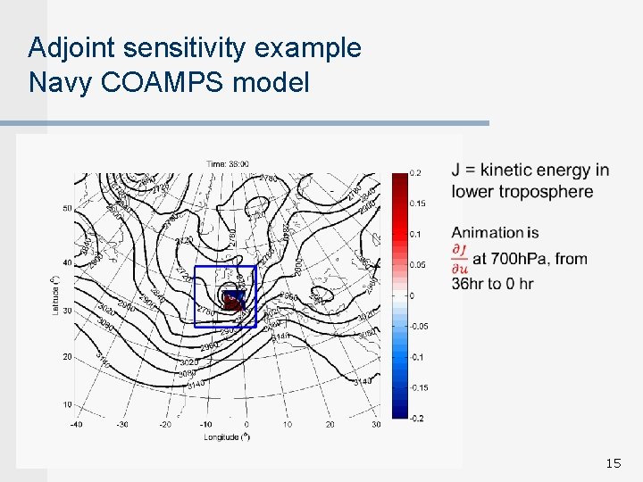
Adjoint sensitivity example Navy COAMPS model 15

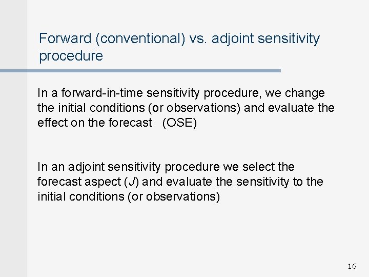
Forward (conventional) vs. adjoint sensitivity procedure In a forward-in-time sensitivity procedure, we change the initial conditions (or observations) and evaluate the effect on the forecast (OSE) In an adjoint sensitivity procedure we select the forecast aspect (J) and evaluate the sensitivity to the initial conditions (or observations) 16

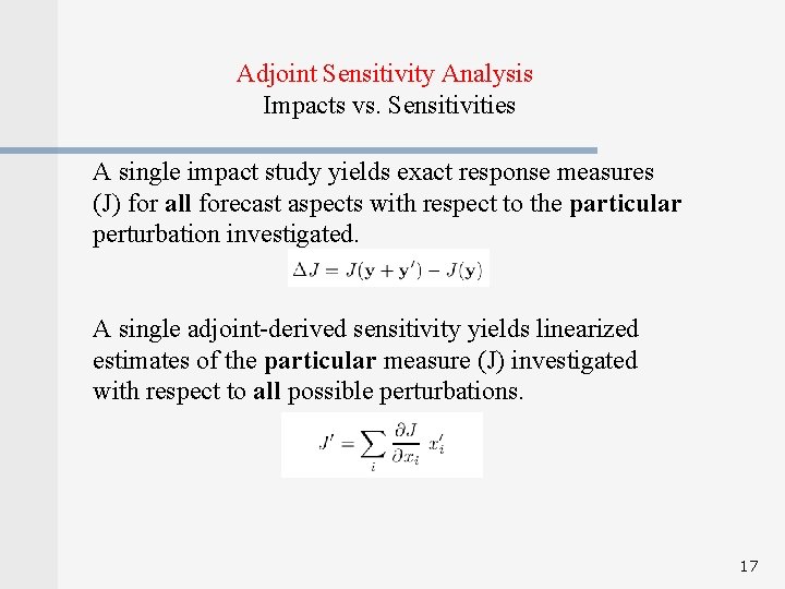
Adjoint Sensitivity Analysis Impacts vs. Sensitivities A single impact study yields exact response measures (J) for all forecast aspects with respect to the particular perturbation investigated. A single adjoint-derived sensitivity yields linearized estimates of the particular measure (J) investigated with respect to all possible perturbations. 17

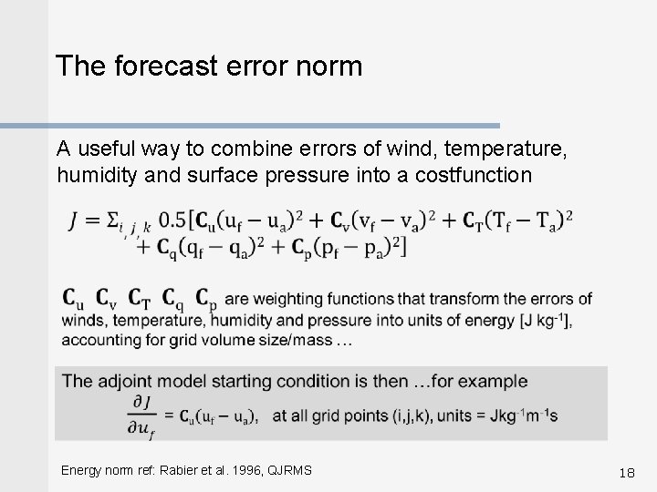
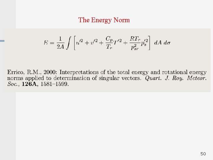
The forecast error norm A useful way to combine errors of wind, temperature, humidity and surface pressure into a costfunction Energy norm ref: Rabier et al. 1996, QJRMS 18

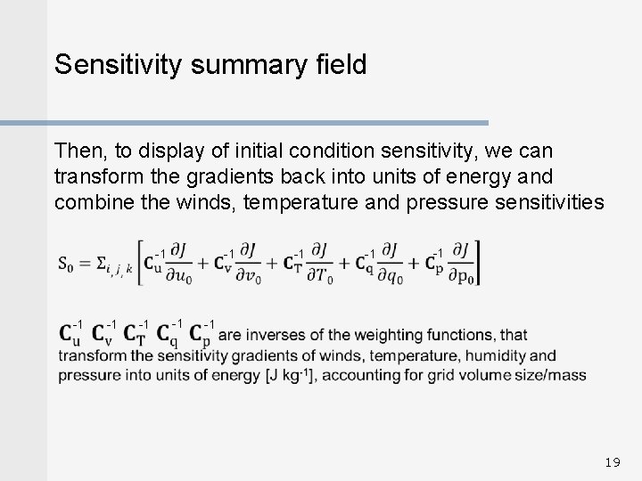
Sensitivity summary field Then, to display of initial condition sensitivity, we can transform the gradients back into units of energy and combine the winds, temperature and pressure sensitivities -1 -1 -1 19

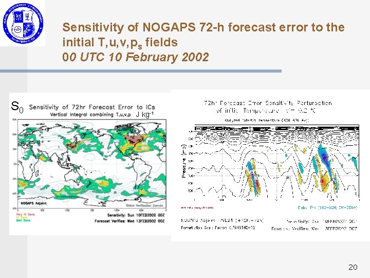
Sensitivity of NOGAPS 72 -h forecast error to the initial T, u, v, ps fields 00 UTC 10 February 2002 S 0 J kg-1 20

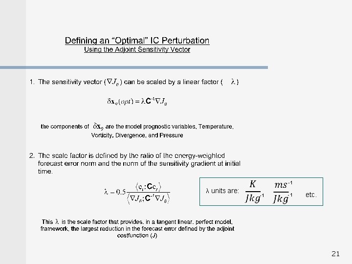
λ units are: -1 -1 -1 etc. 21

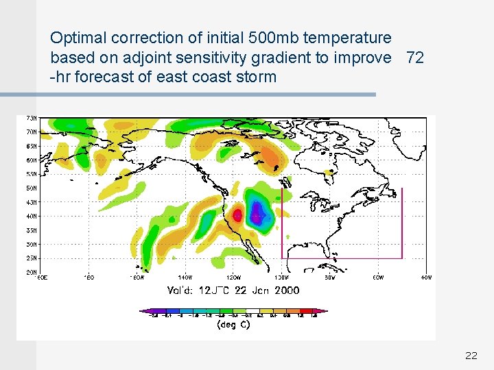
Optimal correction of initial 500 mb temperature based on adjoint sensitivity gradient to improve 72 -hr forecast of east coast storm 22

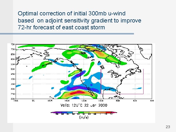
Optimal correction of initial 300 mb u-wind based on adjoint sensitivity gradient to improve 72 -hr forecast of east coast storm 23

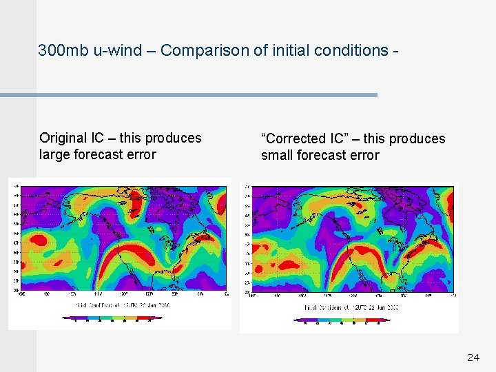
300 mb u-wind – Comparison of initial conditions - Original IC – this produces large forecast error “Corrected IC” – this produces small forecast error 24

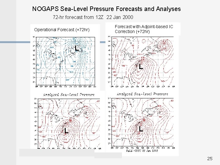
NOGAPS Sea-Level Pressure Forecasts and Analyses 72 -hr forecast from 12 Z 22 Jan 2000 Operational Forecast (+72 hr) Forecast with Adjoint-based IC Correction (+72 hr) L L 25

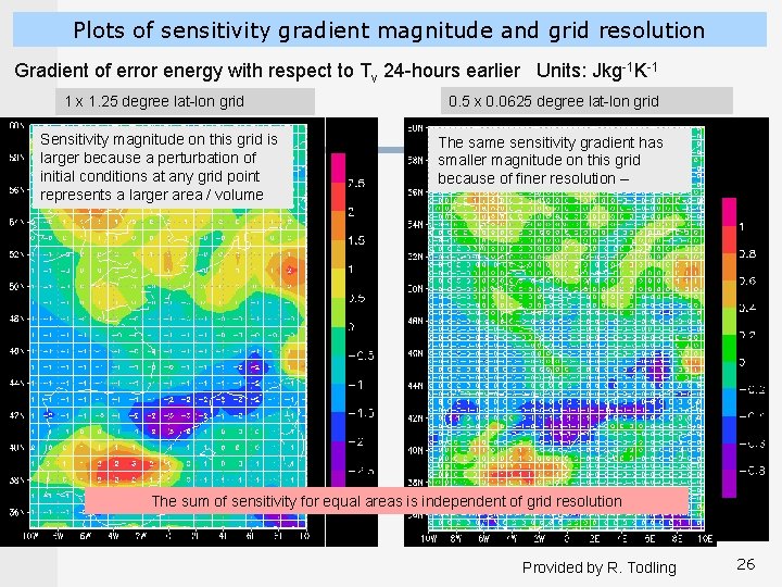
Plots of sensitivity gradient magnitude and grid resolution Gradient of error energy with respect to Tv 24 -hours earlier Units: Jkg-1 K-1 1 x 1. 25 degree lat-lon grid Sensitivity magnitude on this grid is larger because a perturbation of initial conditions at any grid point represents a larger area / volume 0. 5 x 0. 0625 degree lat-lon grid The same sensitivity gradient has smaller magnitude on this grid because of finer resolution – The sum of sensitivity for equal areas is independent of grid resolution Provided by R. Todling 26

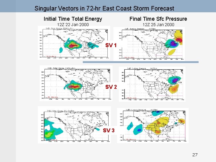
Singular Vectors in 72 -hr East Coast Storm Forecast Initial Time Total Energy Final Time Sfc Pressure 12 Z 22 Jan 2000 12 Z 25 Jan 2000 SV 1 SV 2 SV 3 27

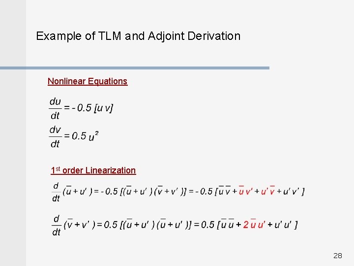
Example of TLM and Adjoint Derivation Nonlinear Equations 1 st order Linearization 28

Example of TLM and Adjoint Derivation Tangent Linear Equations Adjoint Equations (LT) 29

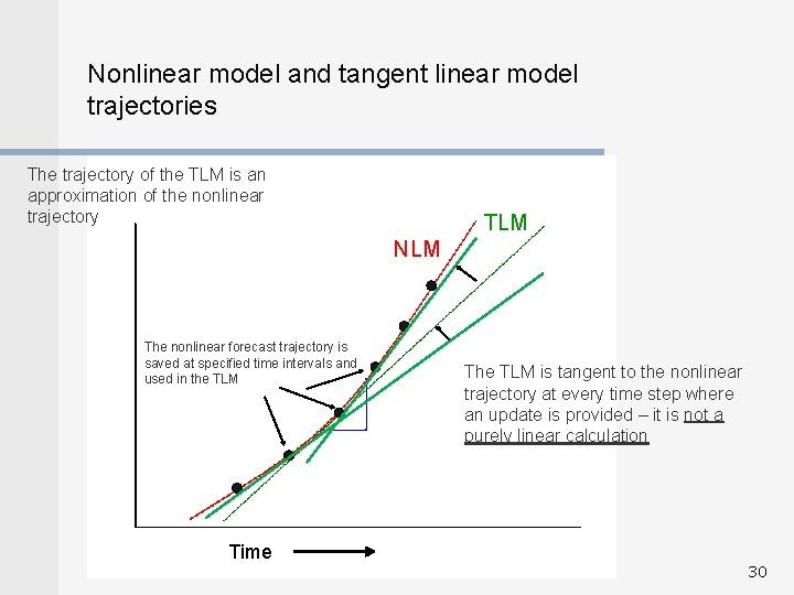
Nonlinear model and tangent linear model trajectories The trajectory of the TLM is an approximation of the nonlinear trajectory TLM NLM The nonlinear forecast trajectory is saved at specified time intervals and used in the TLM Time The TLM is tangent to the nonlinear trajectory at every time step where an update is provided – it is not a purely linear calculation 30

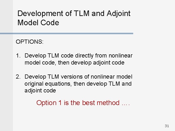
Development of TLM and Adjoint Model Code OPTIONS: 1. Develop TLM code directly from nonlinear model code, then develop adjoint code 2. Develop TLM versions of nonlinear model original equations, then develop TLM and adjoint code Option 1 is the best method …. 31

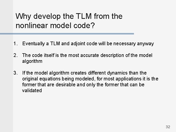
Why develop the TLM from the nonlinear model code? 1. Eventually a TLM and adjoint code will be necessary anyway 2. The code itself is the most accurate description of the model algorithm 3. If the model algorithm creates different dynamics than the original equations being modeled, for most applications it is the former that are desirable and only the former that can be validated 32

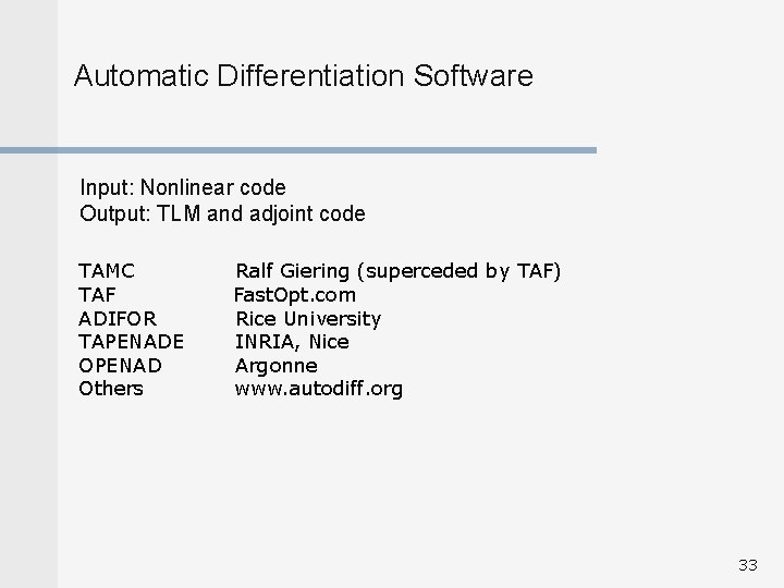
Automatic Differentiation Software Input: Nonlinear code Output: TLM and adjoint code TAMC Ralf Giering (superceded by TAF) TAF Fast. Opt. com ADIFOR Rice University TAPENADE INRIA, Nice OPENAD Argonne Others www. autodiff. org 33

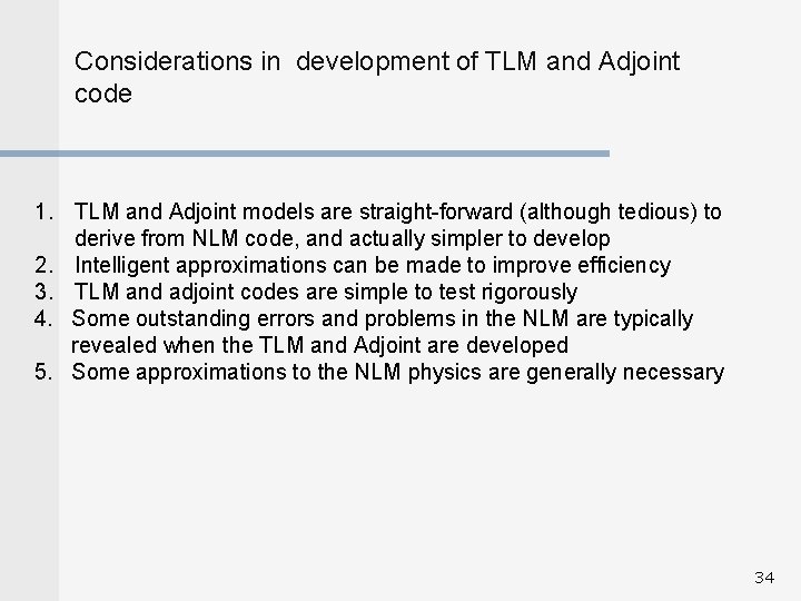
Considerations in development of TLM and Adjoint code 1. TLM and Adjoint models are straight-forward (although tedious) to derive from NLM code, and actually simpler to develop 2. Intelligent approximations can be made to improve efficiency 3. TLM and adjoint codes are simple to test rigorously 4. Some outstanding errors and problems in the NLM are typically revealed when the TLM and Adjoint are developed 5. Some approximations to the NLM physics are generally necessary 34

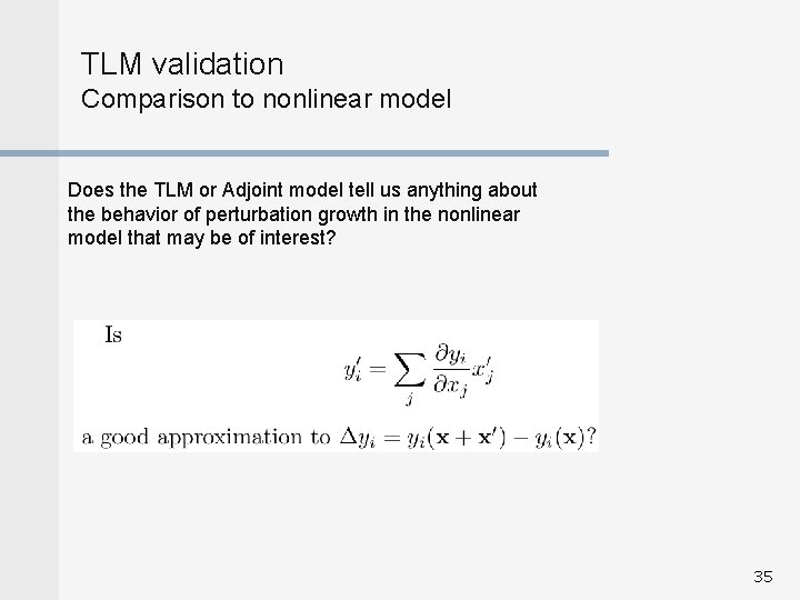
TLM validation Comparison to nonlinear model Does the TLM or Adjoint model tell us anything about the behavior of perturbation growth in the nonlinear model that may be of interest? 35

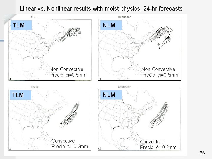
Linear vs. Nonlinear results with moist physics, 24 -hr forecasts TLM Non-Convective Precip. ci=0. 5 mm NLM TLM Convective Precip. ci=0. 2 mm 36

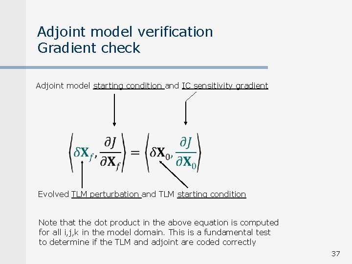
Adjoint model verification Gradient check Adjoint model starting condition and IC sensitivity gradient Evolved TLM perturbation and TLM starting condition Note that the dot product in the above equation is computed for all i, j, k in the model domain. This is a fundamental test to determine if the TLM and adjoint are coded correctly 37

Adjoint method accuracy • Quantitative accuracy best for small perturbations and short forecasts • Often, qualitatively useful information can be obtained for large perturbations in forecasts as long as 3 -5 days…for example, when applied to midlatitude winter storms – synoptic-scales • Accuracy is less for highly non-linear flows and smaller-scales • Adjoint accuracy is equivalent to that of the TLM 38

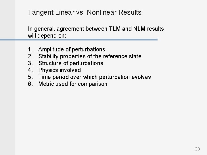
Tangent Linear vs. Nonlinear Results In general, agreement between TLM and NLM results will depend on: 1. 2. 3. 4. 5. 6. Amplitude of perturbations Stability properties of the reference state Structure of perturbations Physics involved Time period over which perturbation evolves Metric used for comparison 39

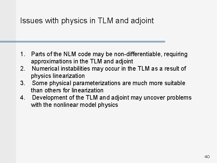
Issues with physics in TLM and adjoint 1. Parts of the NLM code may be non-differentiable, requiring approximations in the TLM and adjoint 2. Numerical instabilities may occur in the TLM as a result of physics linearization 3. Some physical parameterizations are much more suitable than others for linearization 4. Development of the TLM and adjoint may uncover problems with the nonlinear model physics 40

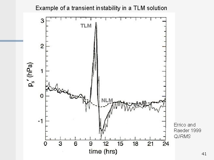
Example of a transient instability in a TLM solution TLM NLM Errico and Raeder 1999 QJRMS 41

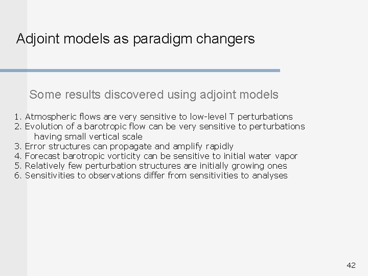
Adjoint models as paradigm changers Some results discovered using adjoint models 1. Atmospheric flows are very sensitive to low-level T perturbations 2. Evolution of a barotropic flow can be very sensitive to perturbations having small vertical scale 3. Error structures can propagate and amplify rapidly 4. Forecast barotropic vorticity can be sensitive to initial water vapor 5. Relatively few perturbation structures are initially growing ones 6. Sensitivities to observations differ from sensitivities to analyses 42

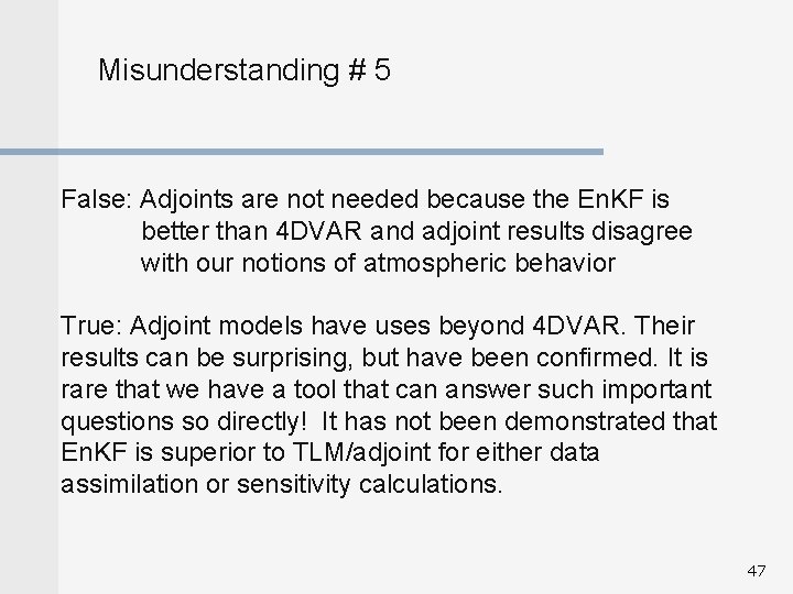
Misunderstanding # 1 False: Adjoint models are difficult to understand True: Understanding how to use and interpret adjoints of numerical models primarily uses concepts taught in early college mathematics 43

Misunderstanding # 2 False: Adjoint models are difficult to develop True: Adjoint models of dynamical cores are simpler to develop than their parent models, and almost trivial to check, but adjoints of model physics can pose difficult problems 44

Misunderstanding # 3 False: Automatic adjoint generators easily generate perfect and useful adjoint models True: Problems can be encountered with automatically generated adjoint codes that are inherent in the parent model. Do these problems also have a bad effect in the parent model? 45

Misunderstanding # 4 False: An adjoint model is demonstrated useful and correct if it reproduces nonlinear results for ranges of very small perturbations True: To be truly useful, adjoint results must yield good approximations to sensitivities with respect to meaningfully large perturbations. This must be part of the validation process 46

Misunderstanding # 5 False: Adjoints are not needed because the En. KF is better than 4 DVAR and adjoint results disagree with our notions of atmospheric behavior True: Adjoint models have uses beyond 4 DVAR. Their results can be surprising, but have been confirmed. It is rare that we have a tool that can answer such important questions so directly! It has not been demonstrated that En. KF is superior to TLM/adjoint for either data assimilation or sensitivity calculations. 47

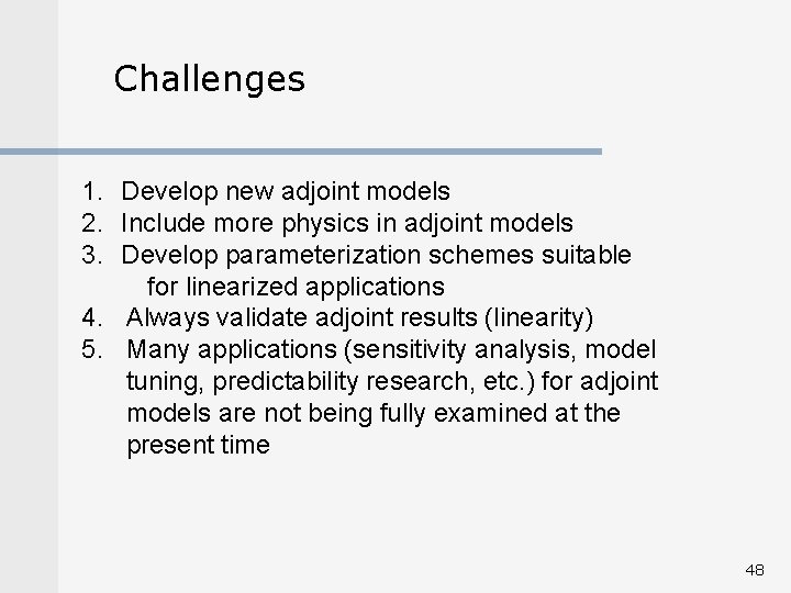
Challenges 1. Develop new adjoint models 2. Include more physics in adjoint models 3. Develop parameterization schemes suitable for linearized applications 4. Always validate adjoint results (linearity) 5. Many applications (sensitivity analysis, model tuning, predictability research, etc. ) for adjoint models are not being fully examined at the present time 48

Adjoint Workshops 1992 – Pacific Grove, CA 1995 – Visegrad, Hungary 1998 – Lennoxville, Quebec 2000 – Moliets-et-Maa, France 2002 – Mount Bethel, PA 2004 – Aquafredda di Maratea, Italy 2006 – Tirol, Austria 2009 – Tannersville, PA 2011 - Cefalu, Sicily 2013? Contact Dr. Ron Errico rerrico@gmao. gsfc. nasa. gov to be put on mailing list 49

The Energy Norm 50