Introduction of Monte Carlo and QuasiMonte Carlo Simulation

Introduction of Monte Carlo and Quasi-Monte Carlo Simulation

Monte Carlo Simulation l Problem Formulation ¤ Given a set of random variables X=(X 1, X 2, … Xn)T and a function of X, Y=f(X), estimate the distribution of the Y l Method ¤ ¤ ¤ Generate N samples of X=(X 1, X 2, … Xn)T For each sample of X, calculate the correspondent sample of Y=f(X) Obtain the distribution of Y from the samples of Y

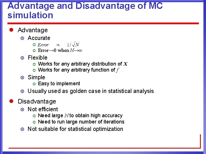
Advantage and Disadvantage of MC simulation l Advantage ¤ Accurate ¢ ¢ ¤ Flexible ¢ ¢ ¤ Works for any arbitrary distribution of X Works for any arbitrary function of f Simple ¢ ¤ Error→ 0 when N→∞ Easy to implement Usually used as golden case in statistical analysis l Disadvantage ¤ Not efficient ¢ ¢ ¤ Need large N to obtain high accuracy Need to run large number of iterations Not suitable for statistical optimization

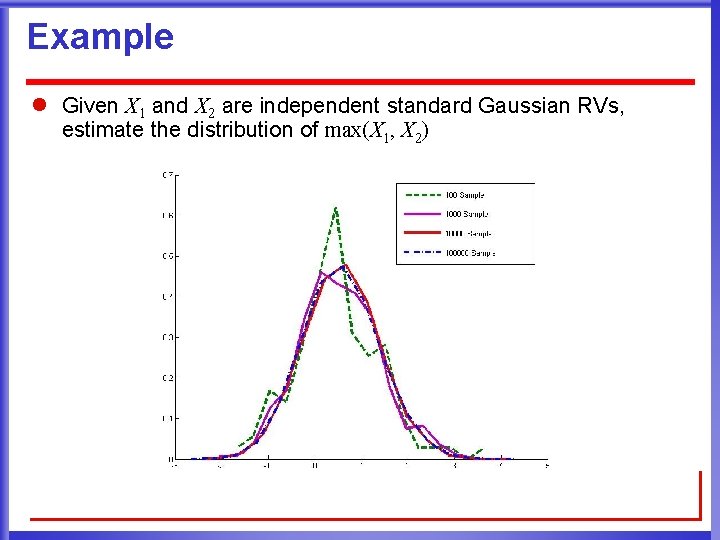
Example l Given X 1 and X 2 are independent standard Gaussian RVs, estimate the distribution of max(X 1, X 2)

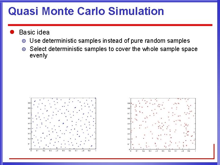
Quasi Monte Carlo Simulation l Basic idea ¤ ¤ Use deterministic samples instead of pure random samples Select deterministic samples to cover the whole sample space evenly

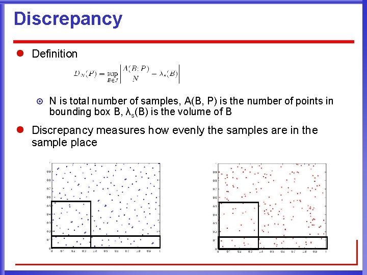
Discrepancy l Definition ¤ N is total number of samples, A(B, P) is the number of points in bounding box B, λs(B) is the volume of B l Discrepancy measures how evenly the samples are in the sample place

Low Discrepancy Sequence l Sample sequence with low discrepancy l Low discrepancy array generation algorithms ¤ ¤ Faure sequence Neiderreiter sequence Sobol sequence Halton Sequence

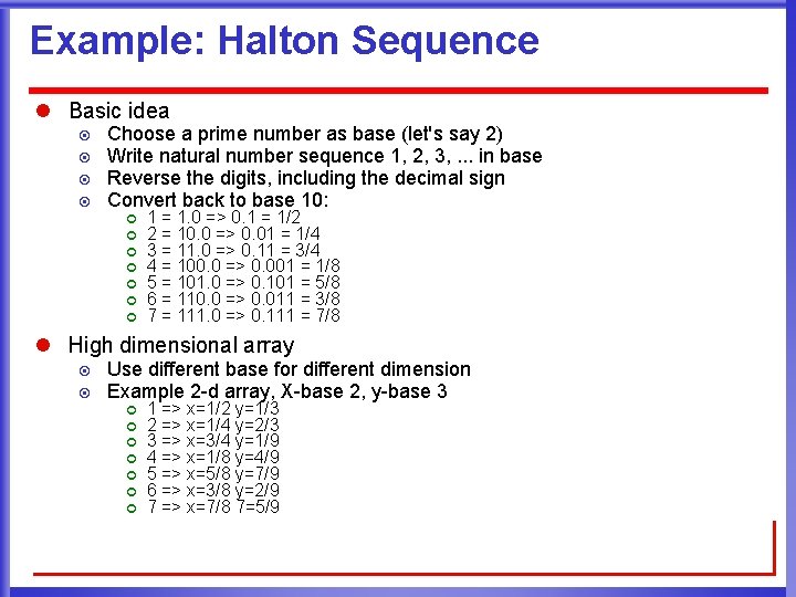
Example: Halton Sequence l Basic idea ¤ ¤ Choose a prime number as base (let's say 2) Write natural number sequence 1, 2, 3, . . . in base Reverse the digits, including the decimal sign Convert back to base 10: ¢ ¢ ¢ ¢ 1 = 1. 0 => 0. 1 = 1/2 2 = 10. 0 => 0. 01 = 1/4 3 = 11. 0 => 0. 11 = 3/4 4 = 100. 0 => 0. 001 = 1/8 5 = 101. 0 => 0. 101 = 5/8 6 = 110. 0 => 0. 011 = 3/8 7 = 111. 0 => 0. 111 = 7/8 l High dimensional array ¤ ¤ Use different base for different dimension Example 2 -d array, X-base 2, y-base 3 ¢ ¢ ¢ ¢ 1 => x=1/2 y=1/3 2 => x=1/4 y=2/3 3 => x=3/4 y=1/9 4 => x=1/8 y=4/9 5 => x=5/8 y=7/9 6 => x=3/8 y=2/9 7 => x=7/8 7=5/9

Advantage and Disadvantage of QMC Simulation l Advantage ¤ Efficient ¢ Use fewer sample than random Monte Carlo simulation l Disadvantage ¤ ¤ ¤ Only works in low dimension cases Very slow when number of random variations become large Not very common in statistical analysis

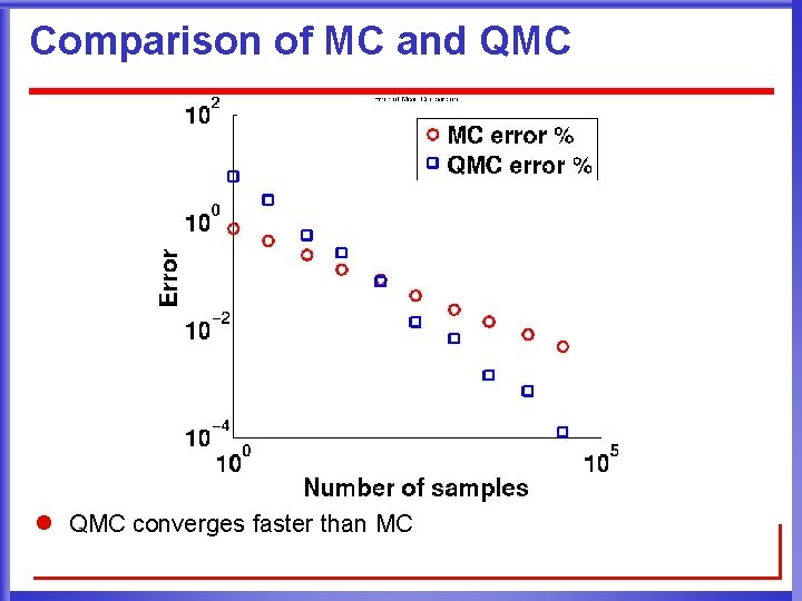
Comparison of MC and QMC l QMC converges faster than MC

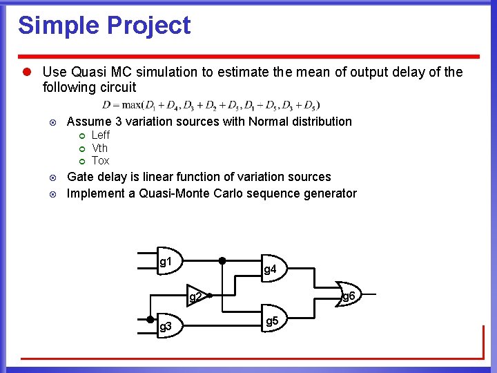
Simple Project l Use Quasi MC simulation to estimate the mean of output delay of the following circuit ¤ Assume 3 variation sources with Normal distribution ¢ ¢ ¢ ¤ ¤ Leff Vth Tox Gate delay is linear function of variation sources Implement a Quasi-Monte Carlo sequence generator g 1 g 4 g 6 g 2 g 3 g 5