Introduction of image segmentation 201716008 Heo Jaeyoung What

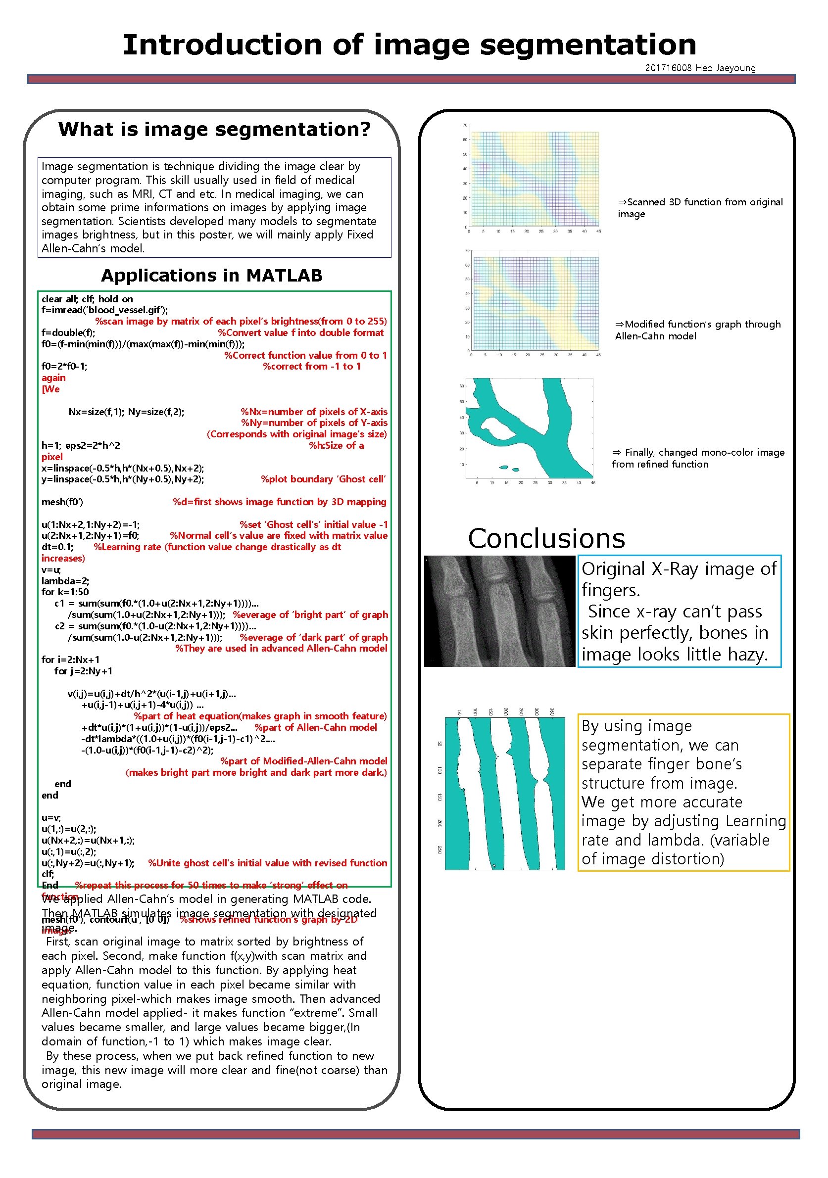
Introduction of image segmentation 201716008 Heo Jaeyoung What is image segmentation? s Image segmentation is technique dividing the image clear by computer program. This skill usually used in field of medical imaging, such as MRI, CT and etc. In medical imaging, we can obtain some prime informations on images by applying image segmentation. Scientists developed many models to segmentate images brightness, but in this poster, we will mainly apply Fixed Allen-Cahn’s model. ⇒Scanned 3 D function from original image Applications in MATLAB clear all; clf; hold on f=imread(‘blood_vessel. gif'); %scan image by matrix of each pixel’s brightness(from 0 to 255) f=double(f); %Convert value f into double format f 0=(f-min(f)))/(max(f))-min(f))); %Correct function value from 0 to 1 f 0=2*f 0 -1; %correct from -1 to 1 again [We Nx=size(f, 1); Ny=size(f, 2); h=1; eps 2=2*h^2 pixel x=linspace(-0. 5*h, h*(Nx+0. 5), Nx+2); y=linspace(-0. 5*h, h*(Ny+0. 5), Ny+2); mesh(f 0') %Nx=number of pixels of X-axis %Ny=number of pixels of Y-axis (Corresponds with original image’s size) %h: Size of a ⇒ Finally, changed mono-color image from refined function %plot boundary ‘Ghost cell’ %d=first shows image function by 3 D mapping u(1: Nx+2, 1: Ny+2)=-1; %set ‘Ghost cell’s’ initial value -1 u(2: Nx+1, 2: Ny+1)=f 0; %Normal cell’s value are fixed with matrix value dt=0. 1; %Learning rate (function value change drastically as dt increases) v=u; lambda=2; for k=1: 50 c 1 = sum(f 0. *(1. 0+u(2: Nx+1, 2: Ny+1)))). . . /sum(1. 0+u(2: Nx+1, 2: Ny+1))); %everage of ‘bright part’ of graph c 2 = sum(f 0. *(1. 0 -u(2: Nx+1, 2: Ny+1)))). . . /sum(1. 0 -u(2: Nx+1, 2: Ny+1))); %everage of ‘dark part’ of graph %They are used in advanced Allen-Cahn model for i=2: Nx+1 for j=2: Ny+1 v(i, j)=u(i, j)+dt/h^2*(u(i-1, j)+u(i+1, j). . . +u(i, j-1)+u(i, j+1)-4*u(i, j)). . . %part of heat equation(makes graph in smooth feature) +dt*u(i, j)*(1+u(i, j))*(1 -u(i, j))/eps 2. . . %part of Allen-Cahn model -dt*lambda*((1. 0+u(i, j))*(f 0(i-1, j-1)-c 1)^2. . -(1. 0 -u(i, j))*(f 0(i-1, j-1)-c 2)^2); %part of Modified-Allen-Cahn model (makes bright part more bright and dark part more dark. ) end u=v; u(1, : )=u(2, : ); u(Nx+2, : )=u(Nx+1, : ); u(: , 1)=u(: , 2); u(: , Ny+2)=u(: , Ny+1); %Unite ghost cell’s initial value with revised function clf; End %repeat this process for 50 times to make ‘strong’ effect on function We applied Allen-Cahn’s model in generating MATLAB code. Then MATLAB simulates image segmentation with designated %shows refined function’s graph by 2 D mesh(f 0'), contourf(u', [0 0]) image. ⇒Modified function’s graph through Allen-Cahn model First, scan original image to matrix sorted by brightness of each pixel. Second, make function f(x, y)with scan matrix and apply Allen-Cahn model to this function. By applying heat equation, function value in each pixel became similar with neighboring pixel-which makes image smooth. Then advanced Allen-Cahn model applied- it makes function “extreme”. Small values became smaller, and large values became bigger, (In domain of function, -1 to 1) which makes image clear. By these process, when we put back refined function to new image, this new image will more clear and fine(not coarse) than original image. Conclusions Original X-Ray image of fingers. Since x-ray can’t pass skin perfectly, bones in image looks little hazy. By using image segmentation, we can separate finger bone’s structure from image. We get more accurate image by adjusting Learning rate and lambda. (variable of image distortion)