Introduction LING 572 Fei Xia Week 1 1306

Introduction LING 572 Fei Xia Week 1: 1/3/06

Outline • Course overview • Problems and methods • Mathematical foundation – Probability theory – Information theory

Course overview

Course objective • Focus on statistical methods that produce stateof-the-art results • Questions: for each algorithm – How the algorithm works: input, output, steps – What kind of tasks an algorithm can be applied to? – How much data is needed? • Labeled data • Unlabeled data

General info • Course website: – Syllabus (incl. slides and papers): updated every week. – Message board – ESubmit • Office hour: W: 3 -5 pm. • Prerequisites: – Ling 570 and Ling 571. – Programming: C, C++, or Java, Perl is a plus. – Introduction to probability and statistics

Expectations • Reading: – Papers are online: who don’t have access to printers? – Reference book: Manning & Schutze (MS) – Finish reading before class. Bring your questions to class. • Grade: – – Homework (3): 30% Project (6 parts): 60% Class participation: 10% No quizzes, exams

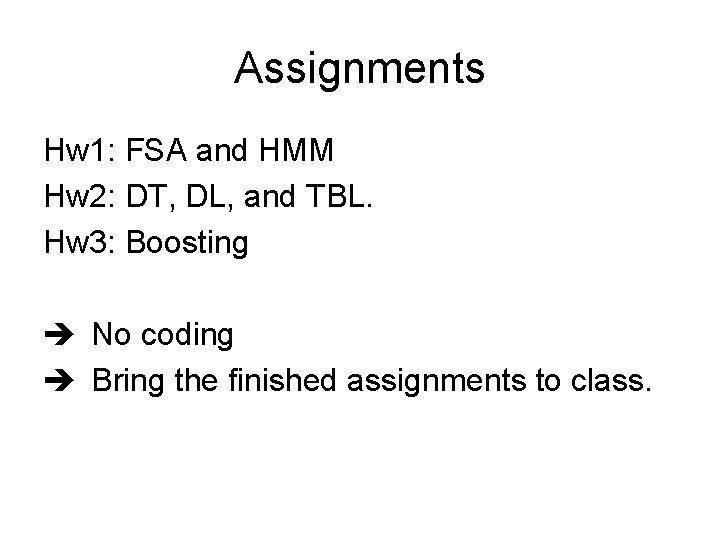
Assignments Hw 1: FSA and HMM Hw 2: DT, DL, and TBL. Hw 3: Boosting No coding Bring the finished assignments to class.

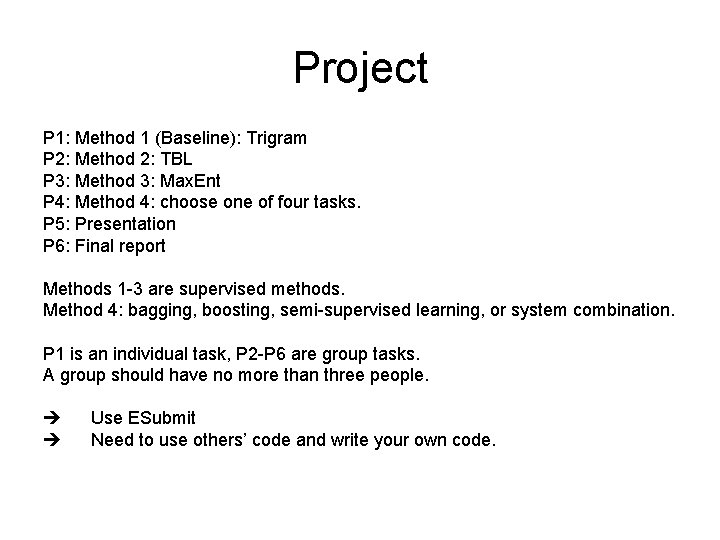
Project P 1: Method 1 (Baseline): Trigram P 2: Method 2: TBL P 3: Method 3: Max. Ent P 4: Method 4: choose one of four tasks. P 5: Presentation P 6: Final report Methods 1 -3 are supervised methods. Method 4: bagging, boosting, semi-supervised learning, or system combination. P 1 is an individual task, P 2 -P 6 are group tasks. A group should have no more than three people. Use ESubmit Need to use others’ code and write your own code.

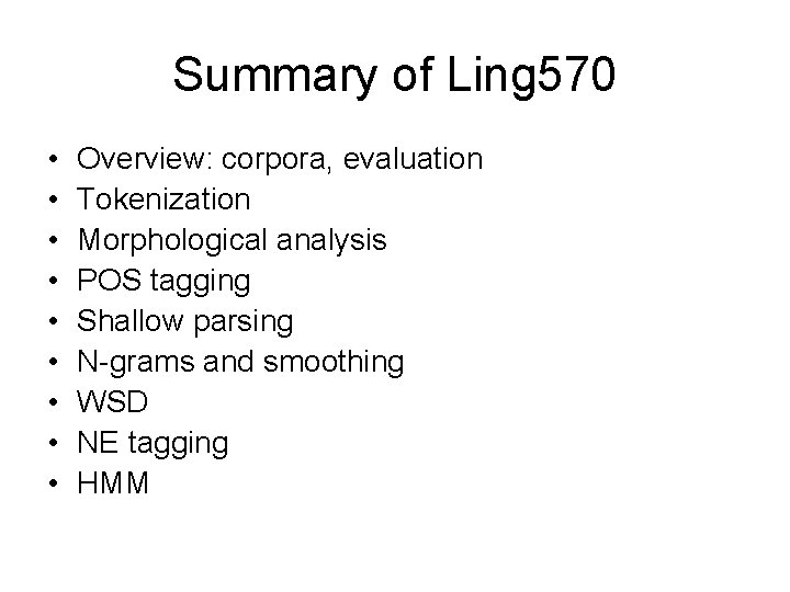
Summary of Ling 570 • • • Overview: corpora, evaluation Tokenization Morphological analysis POS tagging Shallow parsing N-grams and smoothing WSD NE tagging HMM

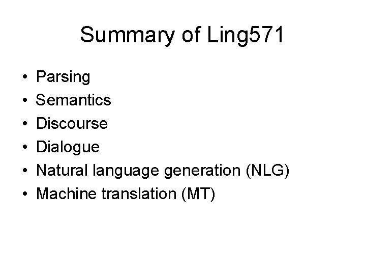
Summary of Ling 571 • • • Parsing Semantics Discourse Dialogue Natural language generation (NLG) Machine translation (MT)

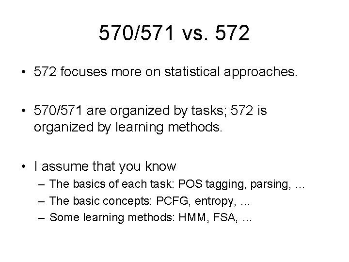
570/571 vs. 572 • 572 focuses more on statistical approaches. • 570/571 are organized by tasks; 572 is organized by learning methods. • I assume that you know – The basics of each task: POS tagging, parsing, … – The basic concepts: PCFG, entropy, … – Some learning methods: HMM, FSA, …

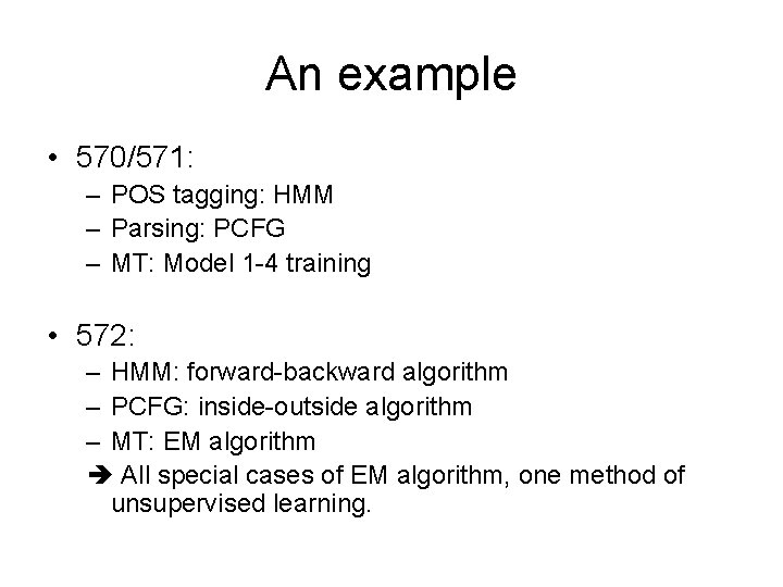
An example • 570/571: – POS tagging: HMM – Parsing: PCFG – MT: Model 1 -4 training • 572: – HMM: forward-backward algorithm – PCFG: inside-outside algorithm – MT: EM algorithm All special cases of EM algorithm, one method of unsupervised learning.

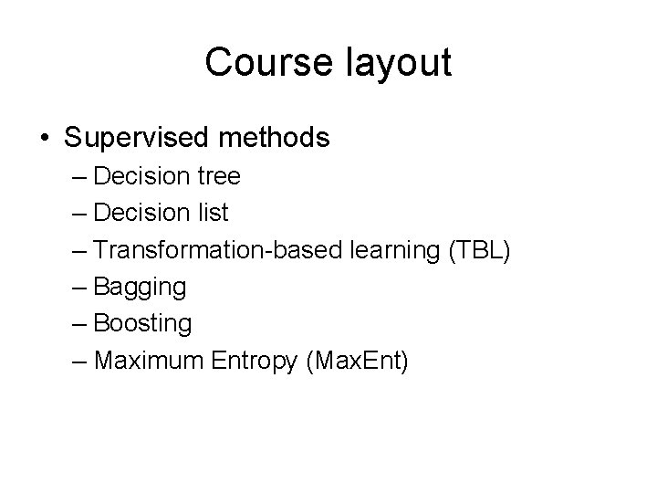
Course layout • Supervised methods – Decision tree – Decision list – Transformation-based learning (TBL) – Bagging – Boosting – Maximum Entropy (Max. Ent)

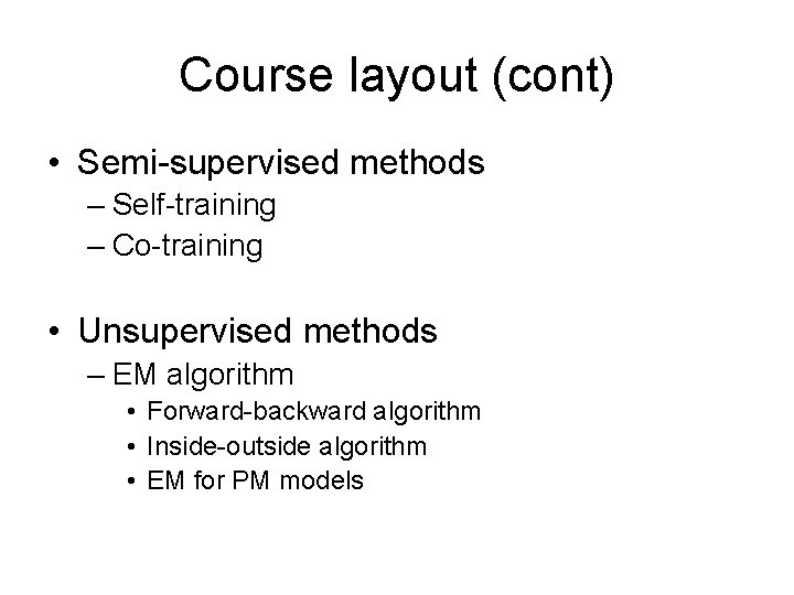
Course layout (cont) • Semi-supervised methods – Self-training – Co-training • Unsupervised methods – EM algorithm • Forward-backward algorithm • Inside-outside algorithm • EM for PM models

Outline • Course overview • Problems and methods • Mathematical foundation – Probability theory – Information theory

Problems and methods

Types of ML problems • • • Classification problem Estimation problem Clustering Discovery … A learning method can be applied to one or more types of ML problems. We will focus on the classification problem.

Classification problem • Given a set of classes and data x, decide which class x belongs to. • Labeled data: – (xi, yi) is a set of labeled data. – xi is a list of attribute values. – yi is a member of a pre-defined set of classes.

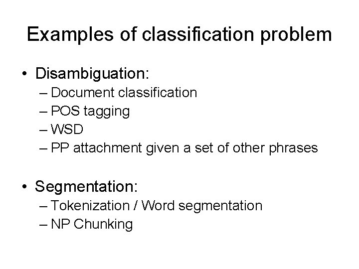
Examples of classification problem • Disambiguation: – Document classification – POS tagging – WSD – PP attachment given a set of other phrases • Segmentation: – Tokenization / Word segmentation – NP Chunking

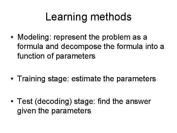
Learning methods • Modeling: represent the problem as a formula and decompose the formula into a function of parameters • Training stage: estimate the parameters • Test (decoding) stage: find the answer given the parameters

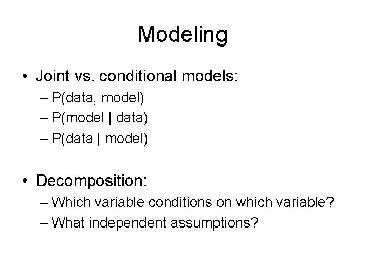
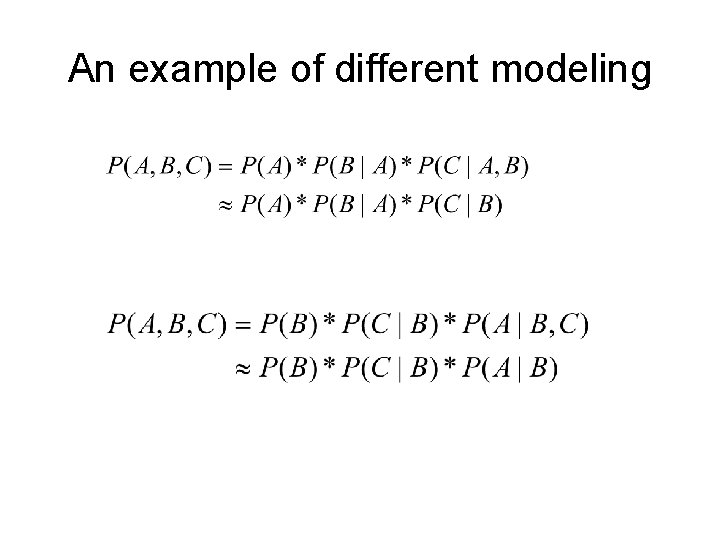
Modeling • Joint vs. conditional models: – P(data, model) – P(model | data) – P(data | model) • Decomposition: – Which variable conditions on which variable? – What independent assumptions?

An example of different modeling

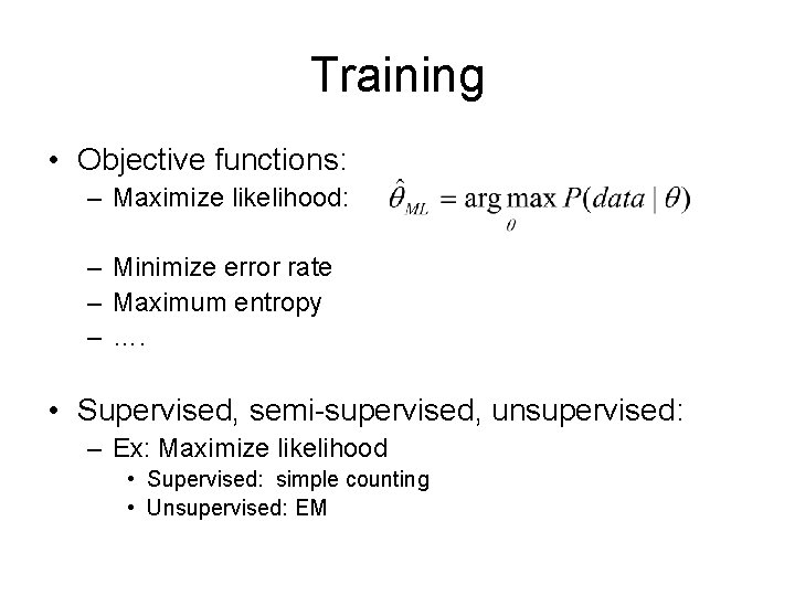
Training • Objective functions: – Maximize likelihood: – Minimize error rate – Maximum entropy – …. • Supervised, semi-supervised, unsupervised: – Ex: Maximize likelihood • Supervised: simple counting • Unsupervised: EM

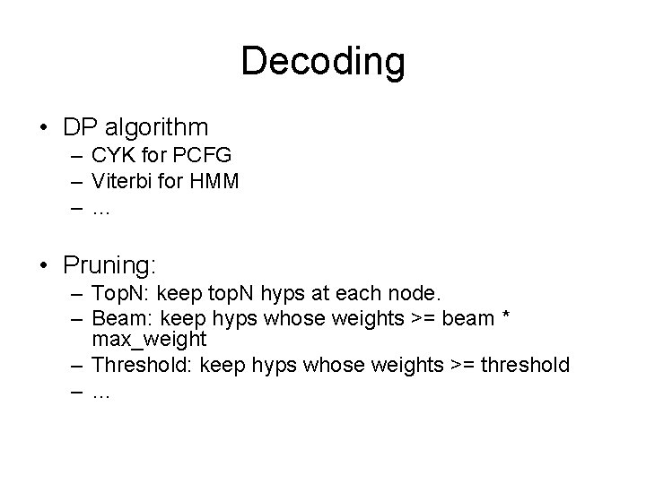
Decoding • DP algorithm – CYK for PCFG – Viterbi for HMM –… • Pruning: – Top. N: keep top. N hyps at each node. – Beam: keep hyps whose weights >= beam * max_weight – Threshold: keep hyps whose weights >= threshold –…

Outline • Course overview • Problems and methods • Mathematical foundation – Probability theory – Information theory

Probability Theory

Probability theory • Sample space, event space • Random variable and random vector • Conditional probability, joint probability, marginal probability (prior)

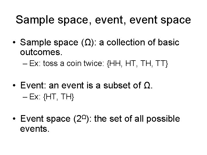
Sample space, event space • Sample space (Ω): a collection of basic outcomes. – Ex: toss a coin twice: {HH, HT, TH, TT} • Event: an event is a subset of Ω. – Ex: {HT, TH} • Event space (2Ω): the set of all possible events.

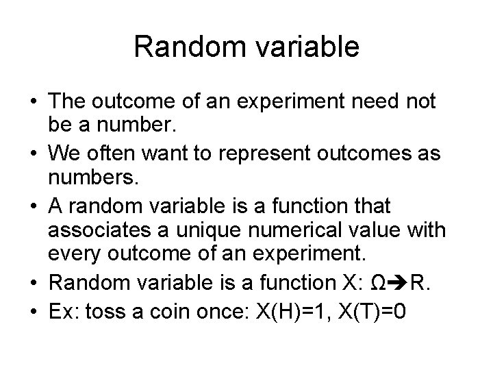
Random variable • The outcome of an experiment need not be a number. • We often want to represent outcomes as numbers. • A random variable is a function that associates a unique numerical value with every outcome of an experiment. • Random variable is a function X: Ω R. • Ex: toss a coin once: X(H)=1, X(T)=0

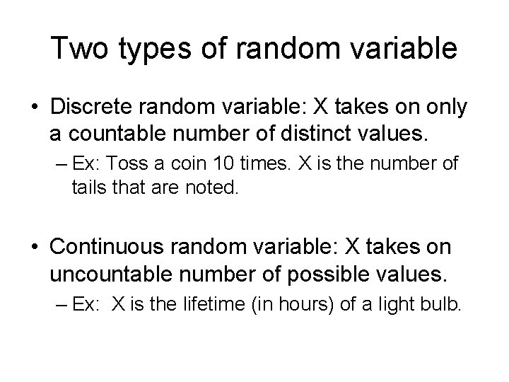
Two types of random variable • Discrete random variable: X takes on only a countable number of distinct values. – Ex: Toss a coin 10 times. X is the number of tails that are noted. • Continuous random variable: X takes on uncountable number of possible values. – Ex: X is the lifetime (in hours) of a light bulb.

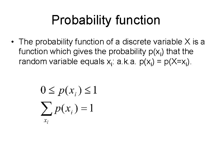
Probability function • The probability function of a discrete variable X is a function which gives the probability p(xi) that the random variable equals xi: a. k. a. p(xi) = p(X=xi).

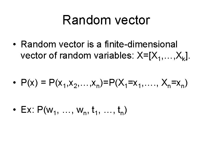
Random vector • Random vector is a finite-dimensional vector of random variables: X=[X 1, …, Xk]. • P(x) = P(x 1, x 2, …, xn)=P(X 1=x 1, …. , Xn=xn) • Ex: P(w 1, …, wn, t 1, …, tn)

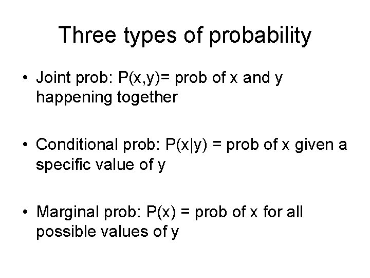
Three types of probability • Joint prob: P(x, y)= prob of x and y happening together • Conditional prob: P(x|y) = prob of x given a specific value of y • Marginal prob: P(x) = prob of x for all possible values of y

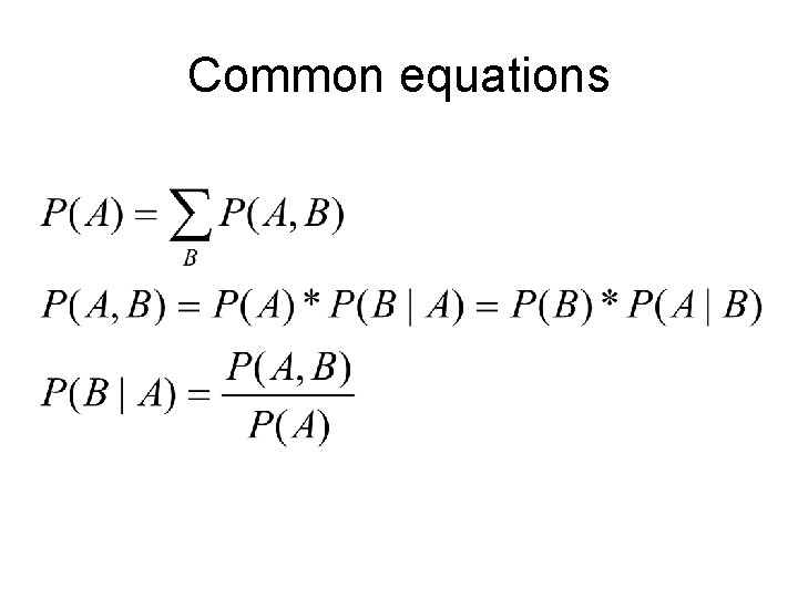
Common equations

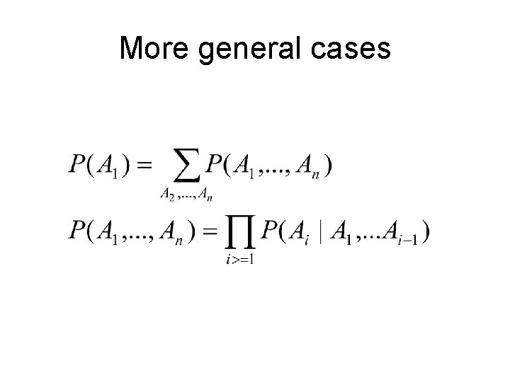
More general cases

Information Theory

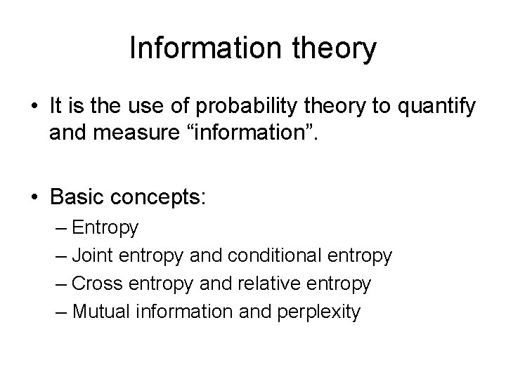
Information theory • It is the use of probability theory to quantify and measure “information”. • Basic concepts: – Entropy – Joint entropy and conditional entropy – Cross entropy and relative entropy – Mutual information and perplexity

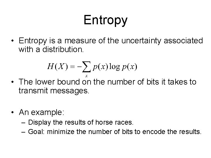
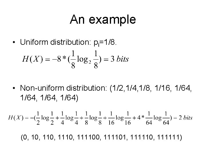
Entropy • Entropy is a measure of the uncertainty associated with a distribution. • The lower bound on the number of bits it takes to transmit messages. • An example: – Display the results of horse races. – Goal: minimize the number of bits to encode the results.

An example • Uniform distribution: pi=1/8. • Non-uniform distribution: (1/2, 1/4, 1/8, 1/16, 1/64, 1/64) (0, 110, 111100, 111101, 111110, 111111)

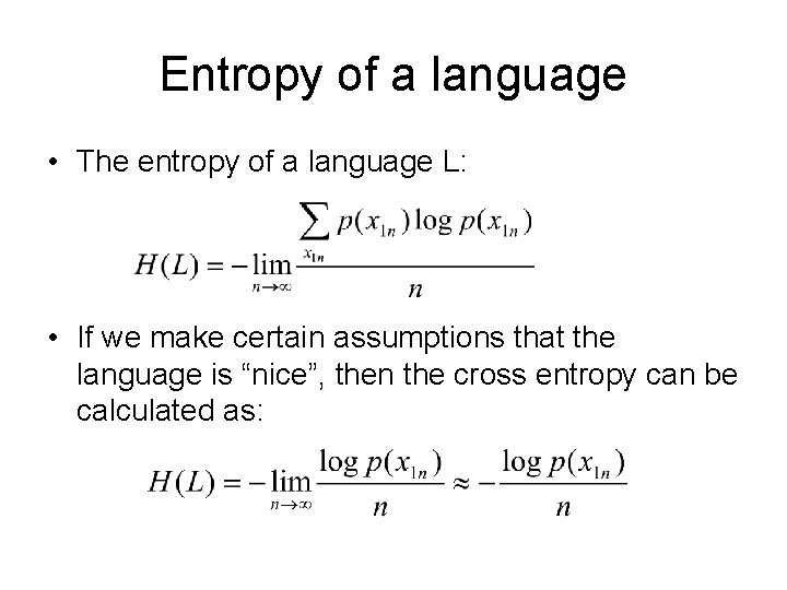
Entropy of a language • The entropy of a language L: • If we make certain assumptions that the language is “nice”, then the cross entropy can be calculated as:

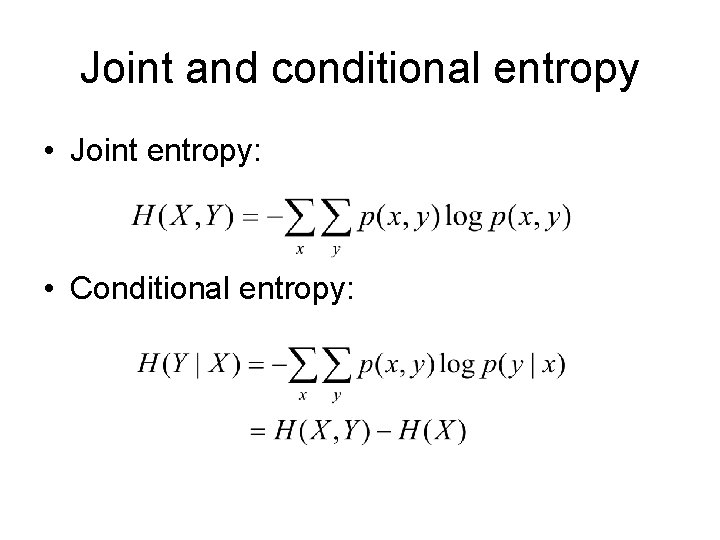
Joint and conditional entropy • Joint entropy: • Conditional entropy:

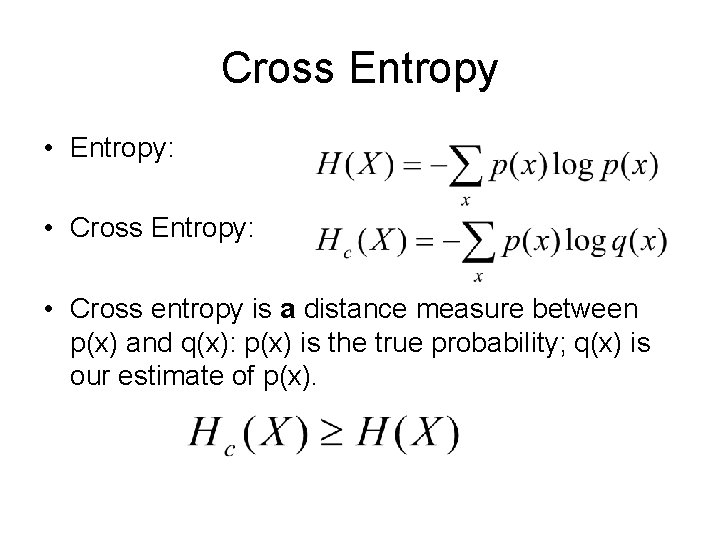
Cross Entropy • Entropy: • Cross entropy is a distance measure between p(x) and q(x): p(x) is the true probability; q(x) is our estimate of p(x).

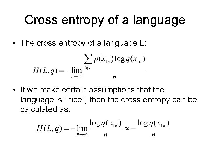
Cross entropy of a language • The cross entropy of a language L: • If we make certain assumptions that the language is “nice”, then the cross entropy can be calculated as:

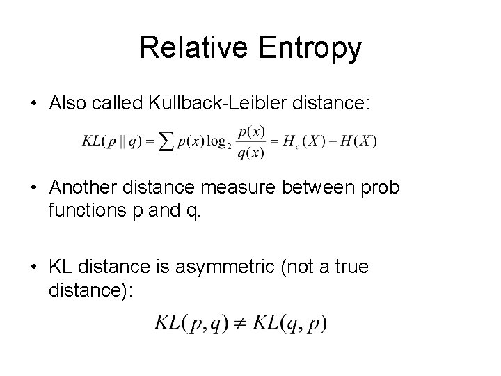
Relative Entropy • Also called Kullback-Leibler distance: • Another distance measure between prob functions p and q. • KL distance is asymmetric (not a true distance):

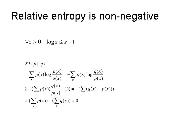
Relative entropy is non-negative

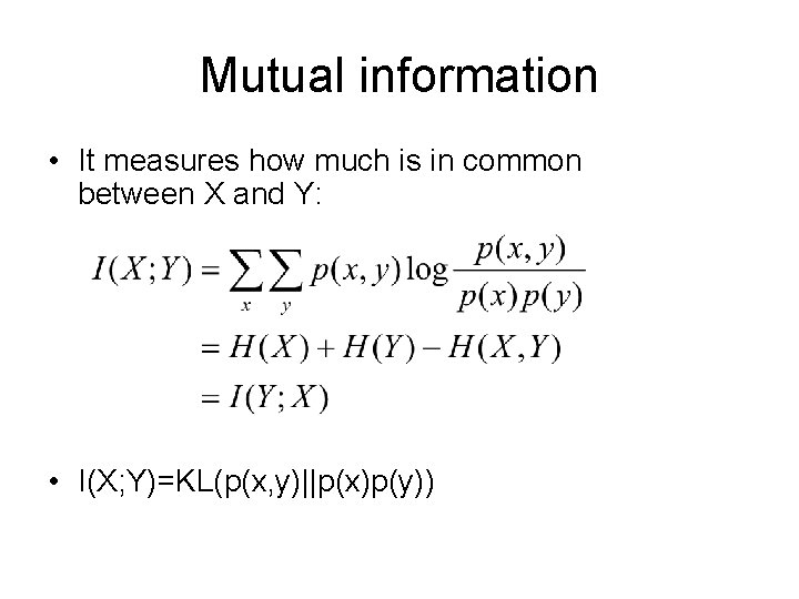
Mutual information • It measures how much is in common between X and Y: • I(X; Y)=KL(p(x, y)||p(x)p(y))

Perplexity • Perplexity is 2 H. • Perplexity is the weighted average number of choices a random variable has to make.

Summary • Course overview • Problems and methods • Mathematical foundation – Probability theory – Information theory M&S Ch 2

Next time • FSA • HMM: M&S Ch 9. 1 and 9. 2