Introduction Introduction and Basic Concept What is Verilog

Introduction

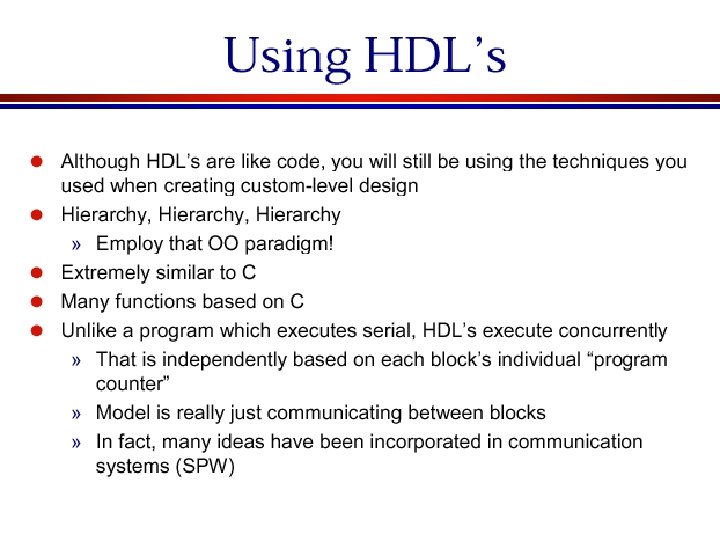
Introduction and Basic Concept • What is Verilog? – Hardware Description Language(HDL) • Why use Verilog? – Because 60% of US companies use it.

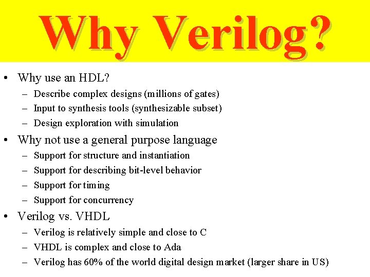
Why Verilog? • Why use an HDL? – Describe complex designs (millions of gates) – Input to synthesis tools (synthesizable subset) – Design exploration with simulation • Why not use a general purpose language – – Support for structure and instantiation Support for describing bit-level behavior Support for timing Support for concurrency • Verilog vs. VHDL – Verilog is relatively simple and close to C – VHDL is complex and close to Ada – Verilog has 60% of the world digital design market (larger share in US)

Why Verilog?

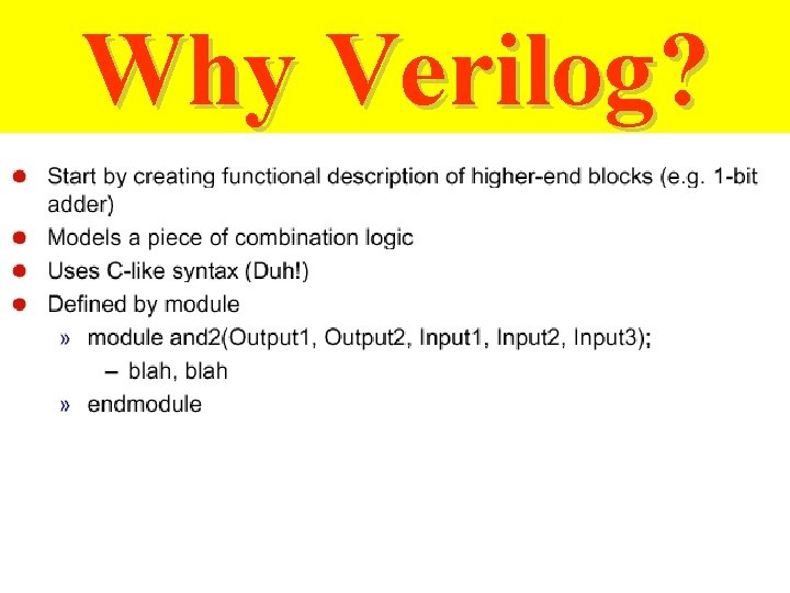
Why Verilog?

Verilog HDL and Verilog-XL • Verilog HDL – Hardware design language that allows you to design circuit. • Verilog-XL – High speed, event-driven simulator that reads Verilog HDL and simulates the behavior of hardware.

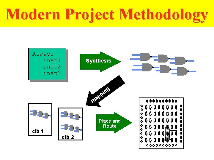
Modern Project Methodology Always inst 1 inst 2 inst 3 Synthesis g in p ap m Place and Route clb 1 clb 2

Introduction to Verilog only • Objectives – Understand the design methodologies using Verilog • Target audience – have basic digital circuits design concept – knowledge of VHDL for design of digital systems – Verilog description for logic synthesis • NOT in the talk – a full coverage of Verilog

Contents • Verilog HDL – structured modeling – RTL modeling • Example combinational circuits – structured description (net-list) – RTL • Example sequential circuits – RTL • FSM – combinational circuits – sequential circuits

Verilog history • Gateway Design Automation – Phil Moorby in 1984 and 1985 • Verilog-XL, "XL algorithm", 1986 – a very efficient method for doing gate-level simulation • Verilog logic synthesizer, Synopsys, 1988 – the top-down design methodology is feasible • Cadence Design Systems acquired Gateway – December 1989 – a proprietary HDL

Verilog history • Open Verilog International (OVI), 1991 – Language Reference Manual (LRM) – making the language specification as vendorindependent as possible. • The IEEE 1364 working group, 1994 – to turn the OVI LRM into an IEEE standard. • Verilog became an IEEE standard – December, 1995.

Hardware Description Languages • The functionality of hardware – concurrency – timing controls • The implementation of hardware – structure – net-list • ISP – C. Gordon Bell and Alan Newell at Carnegie Mellon University, 1972 – RTL (register transfer level)

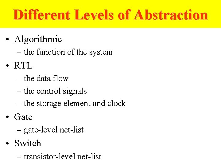
Different Levels of Abstraction • Algorithmic – the function of the system • RTL – the data flow – the control signals – the storage element and clock • Gate – gate-level net-list • Switch – transistor-level net-list

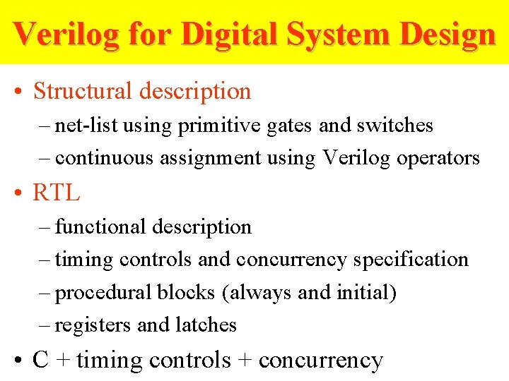
Verilog for Digital System Design • Structural description – net-list using primitive gates and switches – continuous assignment using Verilog operators • RTL – functional description – timing controls and concurrency specification – procedural blocks (always and initial) – registers and latches • C + timing controls + concurrency

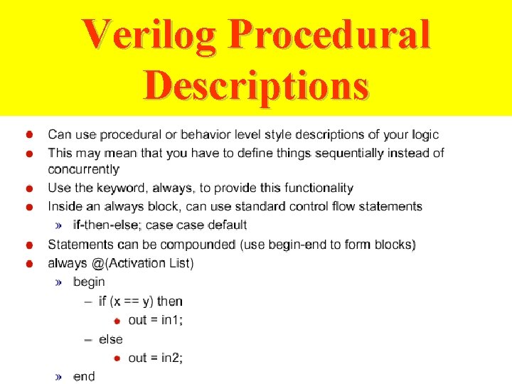
Verilog Procedural Descriptions

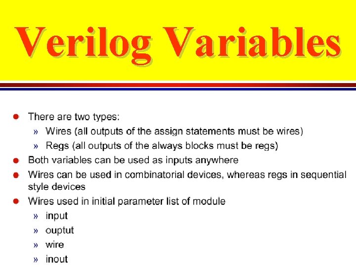
Verilog Variables

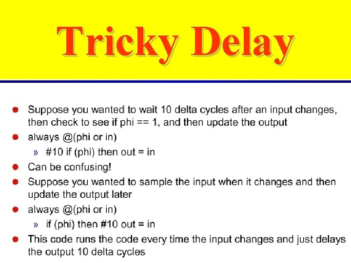
Tricky Delay

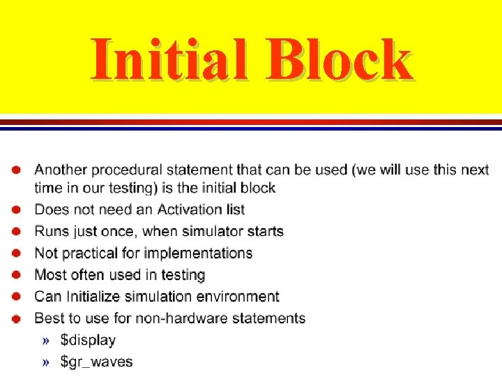
Initial Block

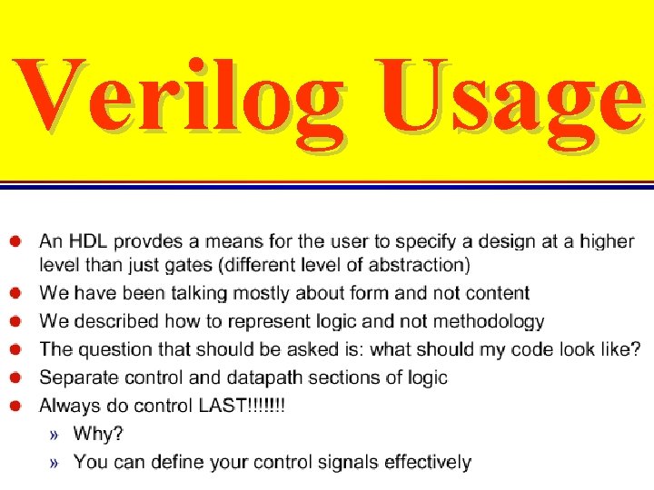
Verilog Usage

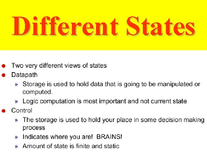
Different States

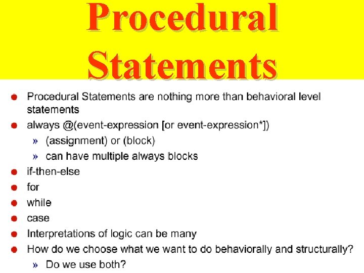
Procedural Statements

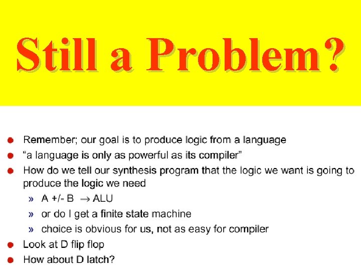
Still a Problem?

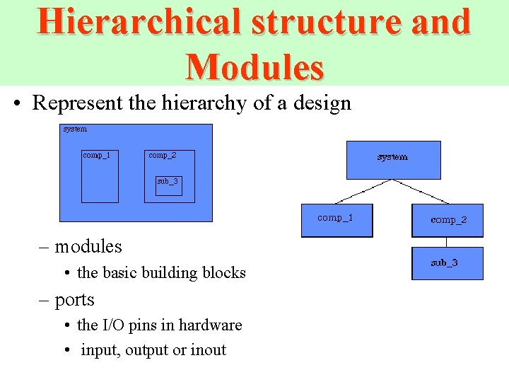
Hierarchical structure and Modules • Represent the hierarchy of a design – modules • the basic building blocks – ports • the I/O pins in hardware • input, output or inout

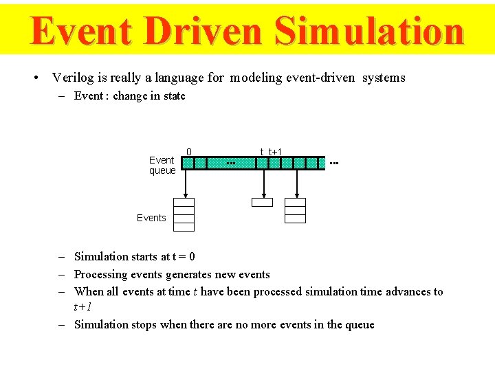
Event Driven Simulation • Verilog is really a language for modeling event-driven systems – Event : change in state Event queue 0 t t+1 • • • Events – Simulation starts at t = 0 – Processing events generates new events – When all events at time t have been processed simulation time advances to t+1 – Simulation stops when there are no more events in the queue

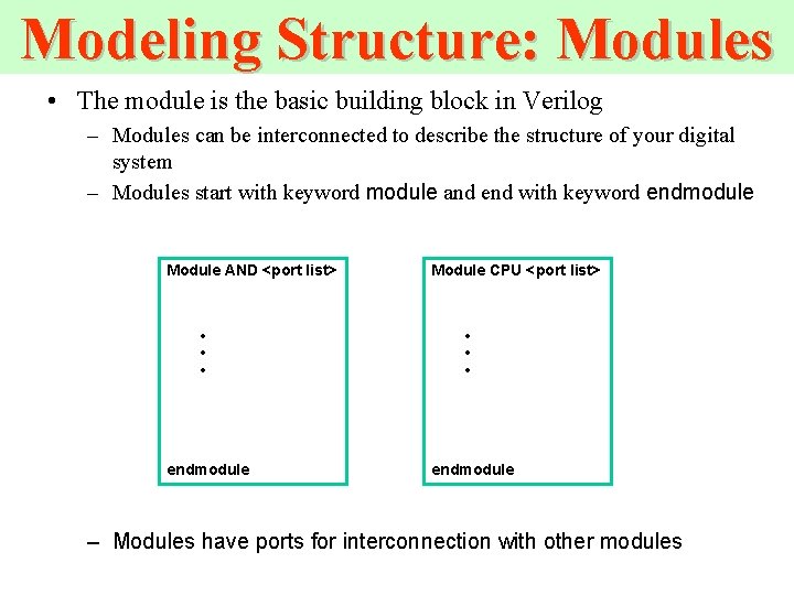
Modeling Structure: Modules • The module is the basic building block in Verilog – Modules can be interconnected to describe the structure of your digital system – Modules start with keyword module and end with keyword endmodule Module AND <port list> Module CPU <port list> • • • endmodule – Modules have ports for interconnection with other modules

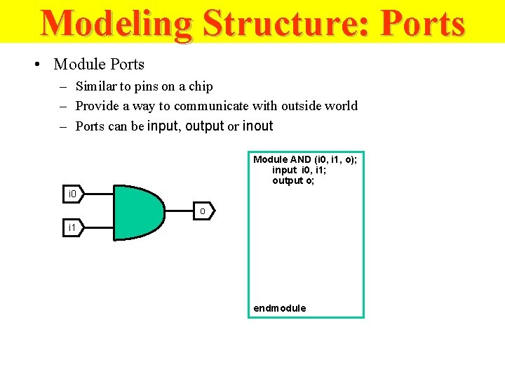
Modeling Structure: Ports • Module Ports – Similar to pins on a chip – Provide a way to communicate with outside world – Ports can be input, output or inout Module AND (i 0, i 1, o); input i 0, i 1; output o; i 0 o i 1 endmodule

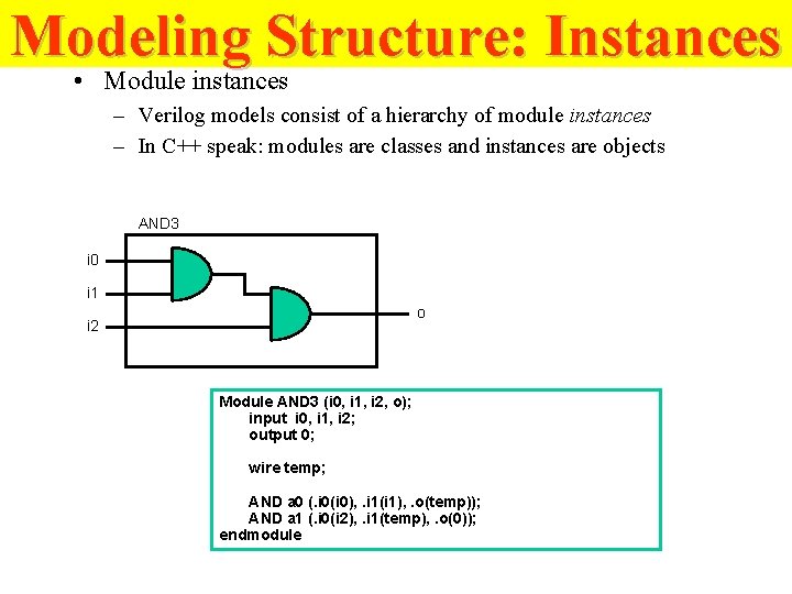
Modeling Structure: Instances • Module instances – Verilog models consist of a hierarchy of module instances – In C++ speak: modules are classes and instances are objects AND 3 i 0 i 1 o i 2 Module AND 3 (i 0, i 1, i 2, o); input i 0, i 1, i 2; output 0; wire temp; AND a 0 (. i 0(i 0), . i 1(i 1), . o(temp)); AND a 1 (. i 0(i 2), . i 1(temp), . o(0)); endmodule

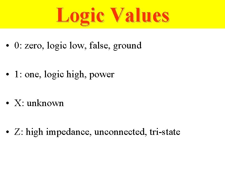
Logic Values • 0: zero, logic low, false, ground • 1: one, logic high, power • X: unknown • Z: high impedance, unconnected, tri-state

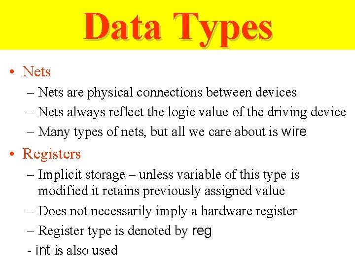
Data Types • Nets – Nets are physical connections between devices – Nets always reflect the logic value of the driving device – Many types of nets, but all we care about is wire • Registers – Implicit storage – unless variable of this type is modified it retains previously assigned value – Does not necessarily imply a hardware register – Register type is denoted by reg - int is also used

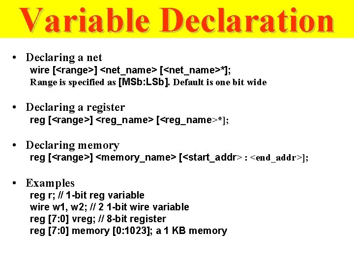
Variable Declaration • Declaring a net wire [<range>] <net_name> [<net_name>*]; Range is specified as [MSb: LSb]. Default is one bit wide • Declaring a register reg [<range>] <reg_name> [<reg_name>*]; • Declaring memory reg [<range>] <memory_name> [<start_addr> : <end_addr>]; • Examples reg r; // 1 -bit reg variable wire w 1, w 2; // 2 1 -bit wire variable reg [7: 0] vreg; // 8 -bit register reg [7: 0] memory [0: 1023]; a 1 KB memory

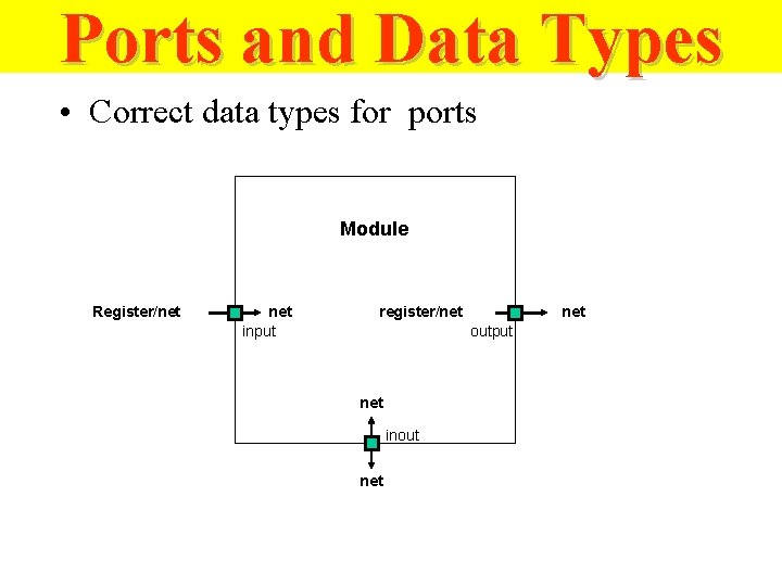
Ports and Data Types • Correct data types for ports Module Register/net input register/net output net inout net

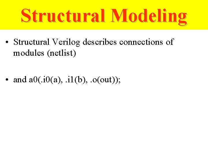
Structural Modeling • Structural Verilog describes connections of modules (netlist) • and a 0(. i 0(a), . i 1(b), . o(out));

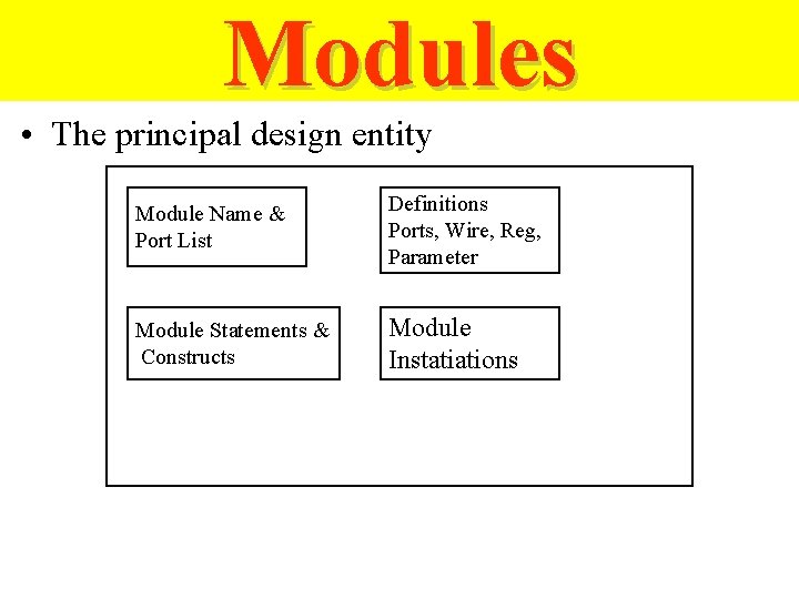
Modules • The principal design entity Module Name & Port List Definitions Ports, Wire, Reg, Parameter Module Statements & Constructs Module Instatiations

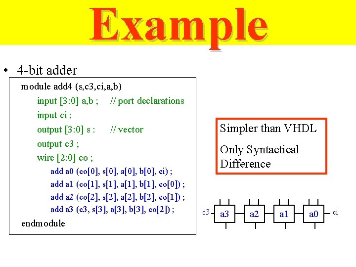
Example • 4 -bit adder module add 4 (s, c 3, ci, a, b) input [3: 0] a, b ; // port declarations input ci ; output [3: 0] s : // vector output c 3 ; wire [2: 0] co ; add a 0 (co[0], s[0], a[0], b[0], ci) ; add a 1 (co[1], s[1], a[1], b[1], co[0]) ; add a 2 (co[2], s[2], a[2], b[2], co[1]) ; add a 3 (c 3, s[3], a[3], b[3], co[2]) ; endmodule Simpler than VHDL Only Syntactical Difference c 3 a 2 a 1 a 0 ci

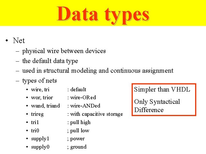
Data types • Net – – physical wire between devices the default data type used in structural modeling and continuous assignment types of nets • wire, tri : default Simpler than VHDL • • wor, trior wand, triand trireg tri 1 tri 0 supply 1 supply 0 : wire-ORed : wire-ANDed : with capacitive storage : pull high ; pull low ; power ; ground Only Syntactical Difference

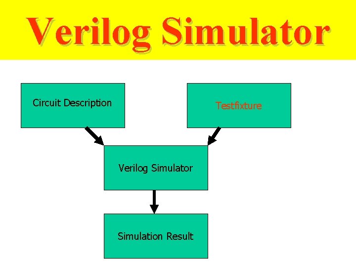
Verilog Simulator Circuit Description Testfixture Verilog Simulator Simulation Result

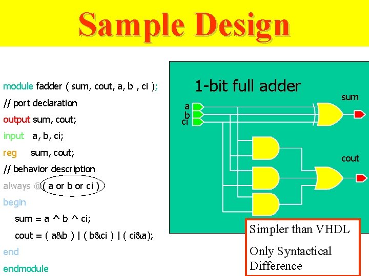
Sample Design 1 -bit full adder module fadder ( sum, cout, a, b , ci ); // port declaration output sum, cout; a b ci sum input a, b, ci; reg sum, cout; cout // behavior description always @( a or b or ci ) begin sum = a ^ b ^ ci; cout = ( a&b ) | ( b&ci ) | ( ci&a); endmodule Simpler than VHDL Only Syntactical Difference

Basic Instructions

Lexical Conventions in Verilog Type of lexical tokens : • Operators ( * ) • White space • Comment • Number ( * ) • String • Identifier • Keyword ( * ) Note : * will be discussed

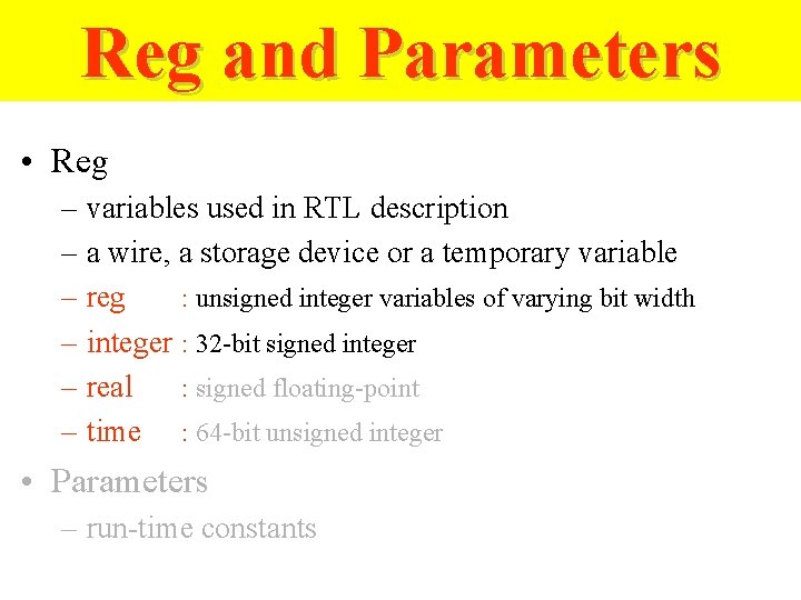
Reg and Parameters • Reg – variables used in RTL description – a wire, a storage device or a temporary variable – reg : unsigned integer variables of varying bit width – integer : 32 -bit signed integer – real : signed floating-point – time : 64 -bit unsigned integer • Parameters – run-time constants

Special Language Tokens • $<identifier>: System tasks and functions – – – – $time $stop $finish $monitor $ps_waves $gr_regs • #<delay specification> – used in • gate instances and procedural statements • unnecessary in RTL specification

Modeling Structures • Net-list – structural description for the top level • Continuous assignments (combination circuits) – data flow specification for simple combinational – Verilog operators • Procedural blocks (RTL) – always and initial blocks • allow timing control and concurrency – C-like procedure statements • primitives (=truth table, state transition table) • function and task (» function and subroutine)

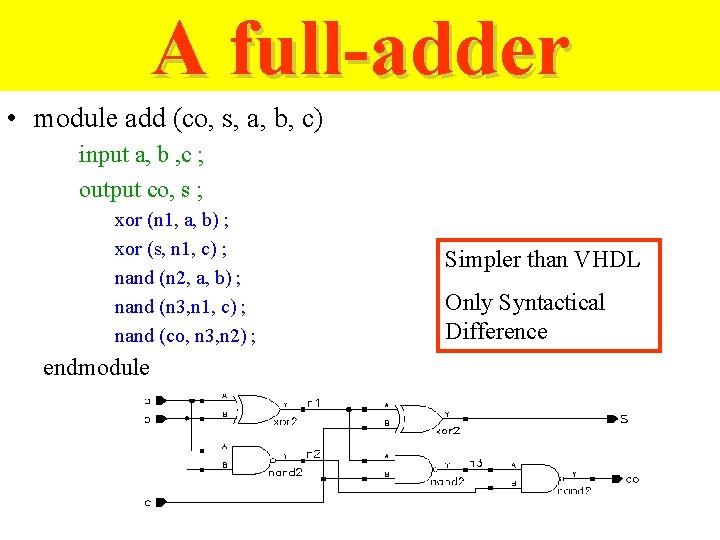
A full-adder • module add (co, s, a, b, c) input a, b , c ; output co, s ; xor (n 1, a, b) ; xor (s, n 1, c) ; nand (n 2, a, b) ; nand (n 3, n 1, c) ; nand (co, n 3, n 2) ; endmodule Simpler than VHDL Only Syntactical Difference

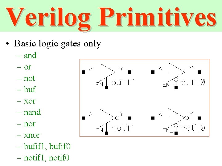
Verilog Primitives • Basic logic gates only – and – or – not – buf – xor – nand – nor – xnor – bufif 1, bufif 0 – notif 1, notif 0

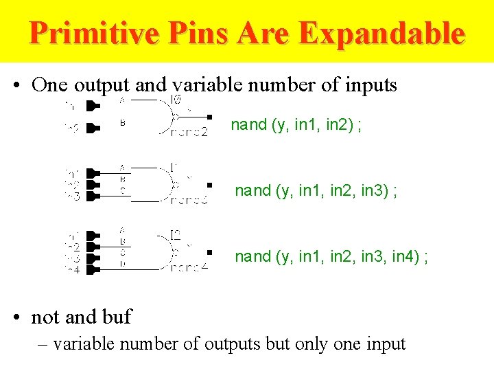
Primitive Pins Are Expandable • One output and variable number of inputs nand (y, in 1, in 2) ; nand (y, in 1, in 2, in 3, in 4) ; • not and buf – variable number of outputs but only one input

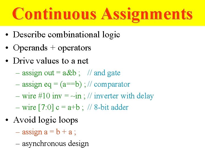
Continuous Assignments • Describe combinational logic • Operands + operators • Drive values to a net – assign out = a&b ; // and gate – assign eq = (a==b) ; // comparator – wire #10 inv = ~in ; // inverter with delay – wire [7: 0] c = a+b ; // 8 -bit adder • Avoid logic loops – assign a = b + a ; – asynchronous design

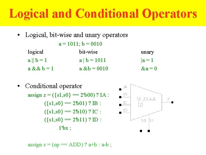
Logical and Conditional Operators • Logical, bit-wise and unary operators a = 1011; b = 0010 logical bit-wise a || b = 1 a | b = 1011 a && b = 1 a &b = 0010 • Conditional operator assign z = ({s 1, s 0} == 2'b 00) ? IA : ({s 1, s 0} == 2'b 01) ? IB : ({s 1, s 0} == 2'b 10) ? IC : ({s 1, s 0} == 2'b 11) ? ID : 1'bx ; assign s = (op == ADD) ? a+b : a-b ; unary |a = 1 &a = 0

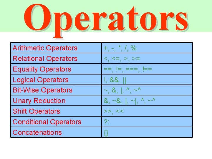
Operators Arithmetic Operators Relational Operators Equality Operators Logical Operators Bit-Wise Operators Unary Reduction Shift Operators Conditional Operators Concatenations +, -, *, /, % <, <=, >, >= ==, !=, ===, !== !, &&, || ~, &, |, ^, ~^ &, ~&, |, ~|, ^, ~^ >>, << ? : {}

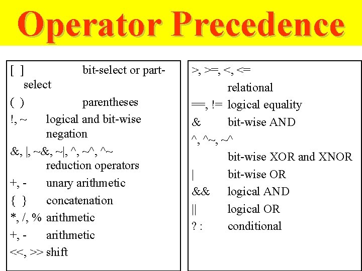
Operator Precedence [ ] bit-select or partselect ( ) parentheses !, ~ logical and bit-wise negation &, |, ~&, ~|, ^, ~^, ^~ reduction operators +, unary arithmetic { } concatenation *, /, % arithmetic +, arithmetic <<, >> shift >, >=, <, <= relational ==, != logical equality & bit-wise AND ^, ^~, ~^ bit-wise XOR and XNOR | bit-wise OR && logical AND || logical OR ? : conditional

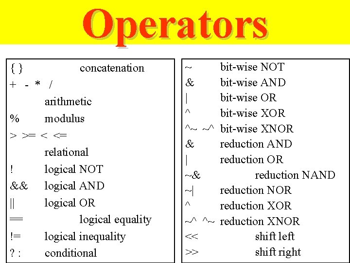
Operators {} concatenation + - * / arithmetic % modulus > >= < <= relational ! logical NOT && logical AND || logical OR == logical equality != logical inequality ? : conditional ~ & | ^ ^~ ~^ & | ~& ~| ^ ~^ ^~ << >> bit-wise NOT bit-wise AND bit-wise OR bit-wise XNOR reduction AND reduction OR reduction NAND reduction NOR reduction XNOR shift left shift right

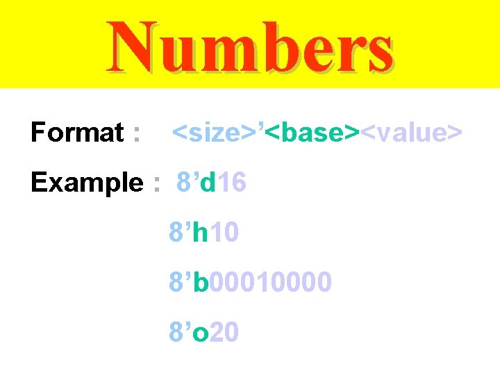
Numbers Format : <size>’<base><value> Example : 8’d 16 8’h 10 8’b 00010000 8’o 20

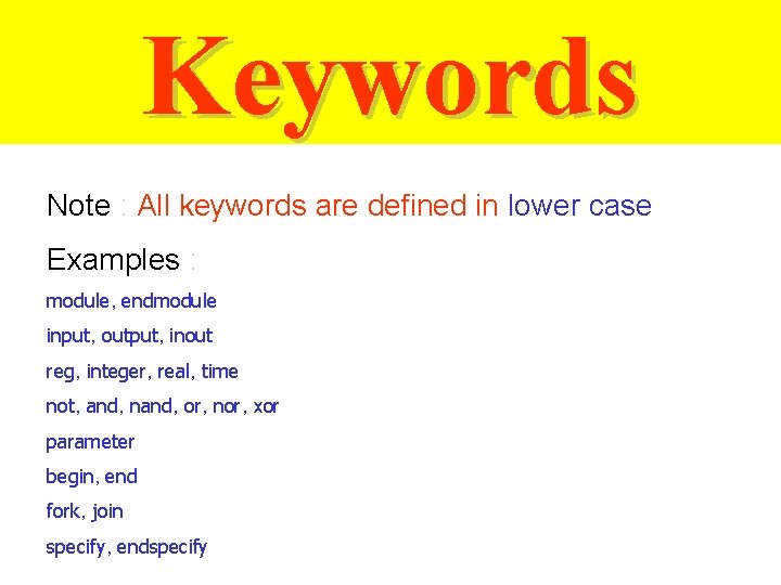
Keywords Note : All keywords are defined in lower case Examples : module, endmodule input, output, inout reg, integer, real, time not, and, nand, or, nor, xor parameter begin, end fork, join specify, endspecify

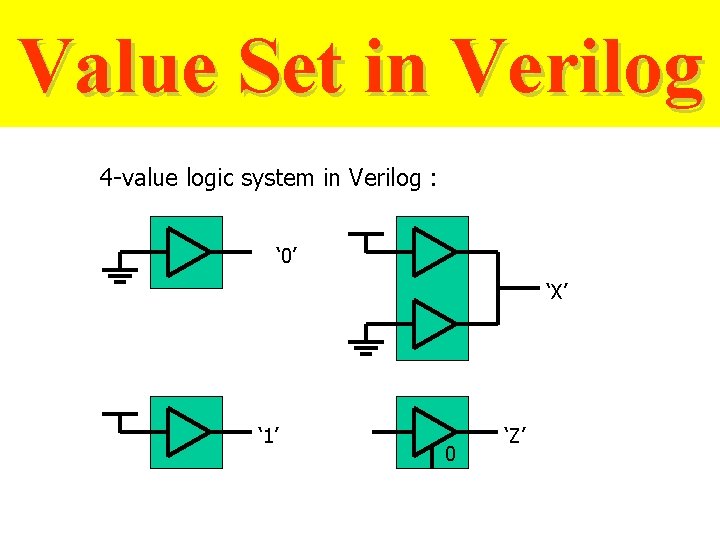
Value Set in Verilog 4 -value logic system in Verilog : ‘ 0’ ‘X’ ‘ 1’ 0 ‘Z’

Major Data Type Class ØNets ØRegisters ØParameters

Nets ØNet data type represent physical connections between structural entities. ØA net must be driven by a driver, such as a gate or a continuous assignment. ØVerilog automatically propagates new values onto a net when the drivers change value.

Registers & Parameters ØRegisters represent abstract storage elements. ØA register holds its value until a new value is assigned to it. ØRegisters are used extensively in behavior modeling and in applying stimuli. ØParameters are not variables, they are constants.

Assignments Assignment : drive values into nets and registers. Continuous Assignments – Any changes in the RHS of continuous assignment are evaluated and the LHS is update. Example : (1) assign out = ~in; (2) assign reg_out; = reg_in << shift

Assignments ( cont. ) Blocking procedural assignment. rega = regb + regc; Non-blocking procedural assignment. rega <= regb * regc;

RTL Modeling

RTL Modeling • Describe the system at a high level of abstraction • Specify a set of concurrently active procedural blocks – procedural blocks = digital circuits • Procedural blocks – initial blocks • test-fixtures to generate test vectors • initial conditions – always blocks • can be combinational circuits • can imply latches or flip-flops

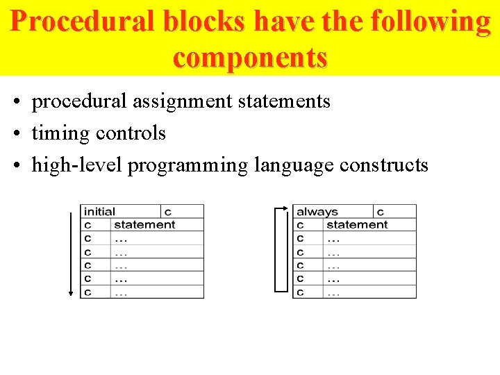
Procedural blocks have the following components • procedural assignment statements • timing controls • high-level programming language constructs

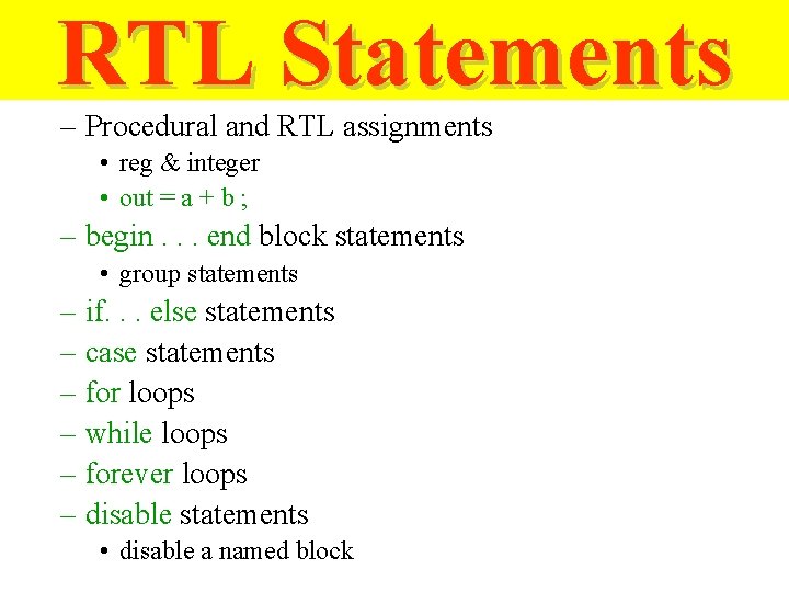
RTL Statements – Procedural and RTL assignments • reg & integer • out = a + b ; – begin. . . end block statements • group statements – if. . . else statements – case statements – for loops – while loops – forever loops – disable statements • disable a named block

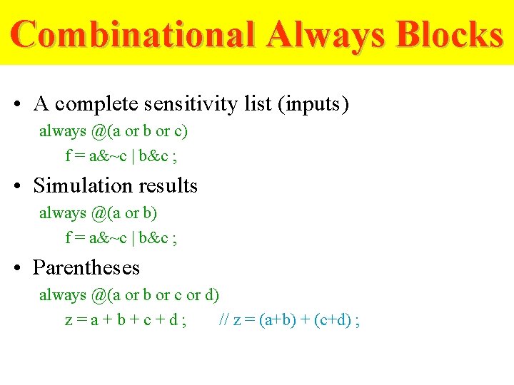
Combinational Always Blocks • A complete sensitivity list (inputs) always @(a or b or c) f = a&~c | b&c ; • Simulation results always @(a or b) f = a&~c | b&c ; • Parentheses always @(a or b or c or d) z=a+b+c+d; // z = (a+b) + (c+d) ;

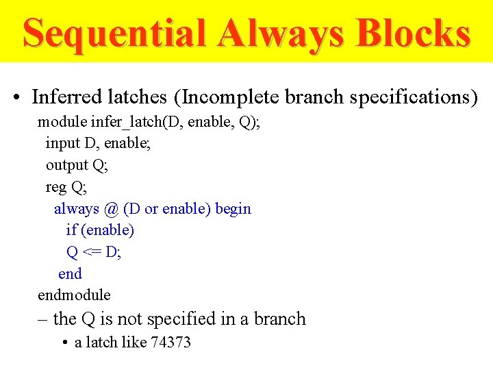
Sequential Always Blocks • Inferred latches (Incomplete branch specifications) module infer_latch(D, enable, Q); input D, enable; output Q; reg Q; always @ (D or enable) begin if (enable) Q <= D; endmodule – the Q is not specified in a branch • a latch like 74373

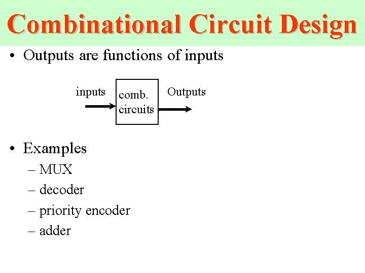
Combinational Circuit Design • Outputs are functions of inputs comb. circuits • Examples – MUX – decoder – priority encoder – adder Outputs

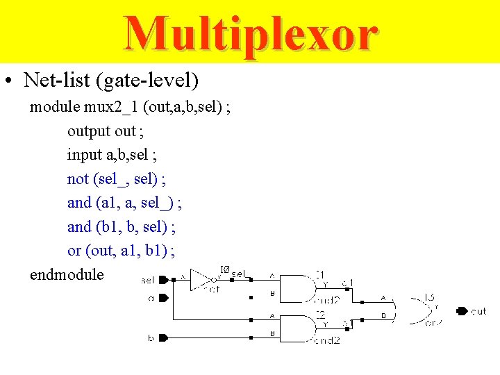
Multiplexor • Net-list (gate-level) module mux 2_1 (out, a, b, sel) ; output out ; input a, b, sel ; not (sel_, sel) ; and (a 1, a, sel_) ; and (b 1, b, sel) ; or (out, a 1, b 1) ; endmodule

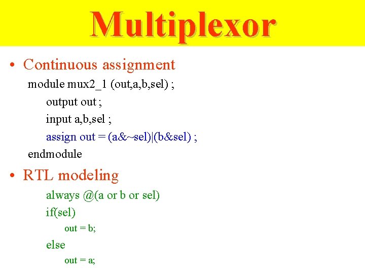
Multiplexor • Continuous assignment module mux 2_1 (out, a, b, sel) ; output out ; input a, b, sel ; assign out = (a&~sel)|(b&sel) ; endmodule • RTL modeling always @(a or b or sel) if(sel) out = b; else out = a;

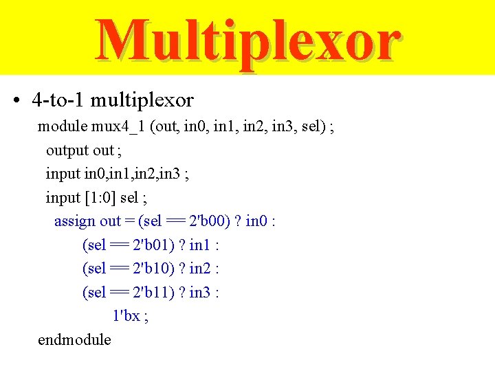
Multiplexor • 4 -to-1 multiplexor module mux 4_1 (out, in 0, in 1, in 2, in 3, sel) ; output out ; input in 0, in 1, in 2, in 3 ; input [1: 0] sel ; assign out = (sel == 2'b 00) ? in 0 : (sel == 2'b 01) ? in 1 : (sel == 2'b 10) ? in 2 : (sel == 2'b 11) ? in 3 : 1'bx ; endmodule

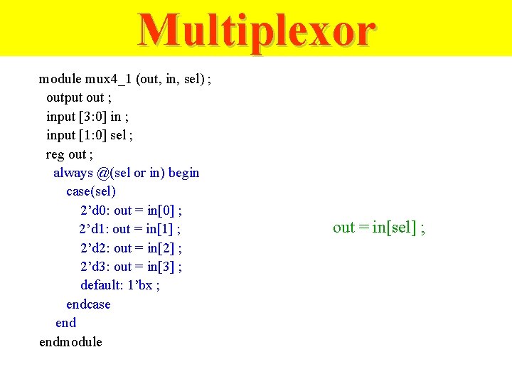
Multiplexor module mux 4_1 (out, in, sel) ; output out ; input [3: 0] in ; input [1: 0] sel ; reg out ; always @(sel or in) begin case(sel) 2’d 0: out = in[0] ; 2’d 1: out = in[1] ; 2’d 2: out = in[2] ; 2’d 3: out = in[3] ; default: 1’bx ; endcase endmodule out = in[sel] ;

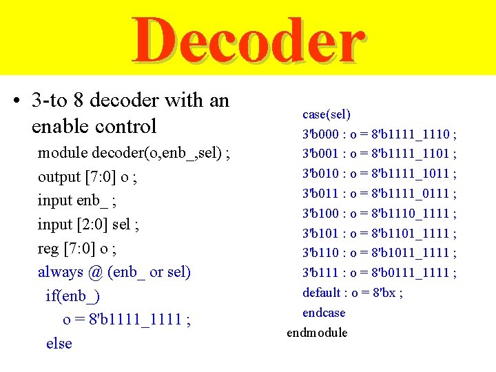
Decoder • 3 -to 8 decoder with an enable control module decoder(o, enb_, sel) ; output [7: 0] o ; input enb_ ; input [2: 0] sel ; reg [7: 0] o ; always @ (enb_ or sel) if(enb_) o = 8'b 1111_1111 ; else case(sel) 3'b 000 : o = 8'b 1111_1110 ; 3'b 001 : o = 8'b 1111_1101 ; 3'b 010 : o = 8'b 1111_1011 ; 3'b 011 : o = 8'b 1111_0111 ; 3'b 100 : o = 8'b 1110_1111 ; 3'b 101 : o = 8'b 1101_1111 ; 3'b 110 : o = 8'b 1011_1111 ; 3'b 111 : o = 8'b 0111_1111 ; default : o = 8'bx ; endcase endmodule

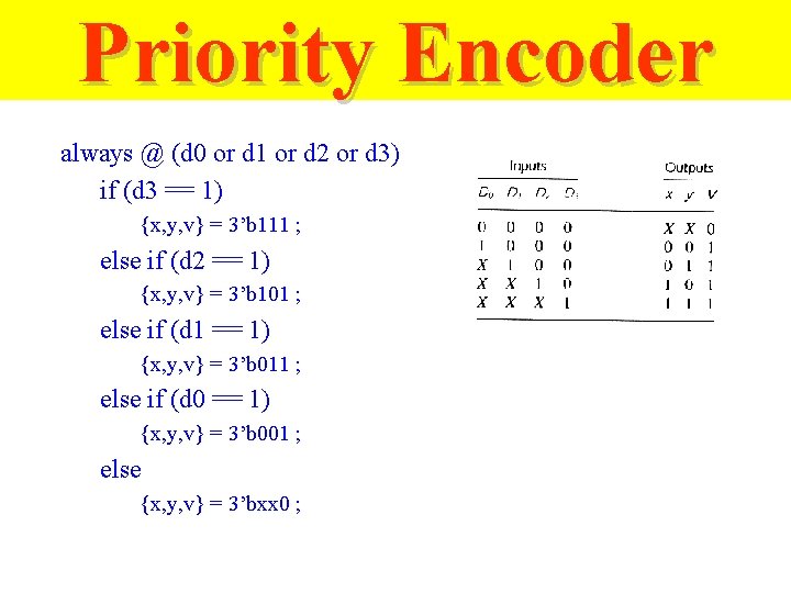
Priority Encoder always @ (d 0 or d 1 or d 2 or d 3) if (d 3 == 1) {x, y, v} = 3’b 111 ; else if (d 2 == 1) {x, y, v} = 3’b 101 ; else if (d 1 == 1) {x, y, v} = 3’b 011 ; else if (d 0 == 1) {x, y, v} = 3’b 001 ; else {x, y, v} = 3’bxx 0 ;

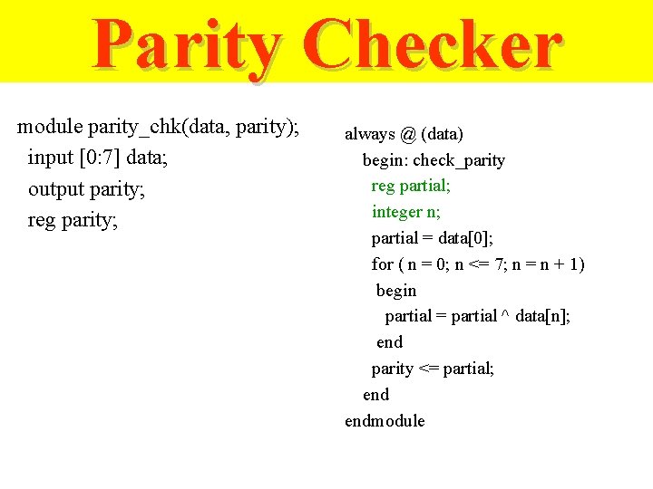
Parity Checker module parity_chk(data, parity); input [0: 7] data; output parity; reg parity; always @ (data) begin: check_parity reg partial; integer n; partial = data[0]; for ( n = 0; n <= 7; n = n + 1) begin partial = partial ^ data[n]; end parity <= partial; endmodule

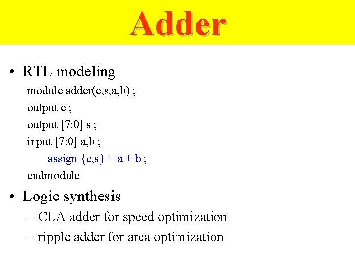
Adder • RTL modeling module adder(c, s, a, b) ; output c ; output [7: 0] s ; input [7: 0] a, b ; assign {c, s} = a + b ; endmodule • Logic synthesis – CLA adder for speed optimization – ripple adder for area optimization

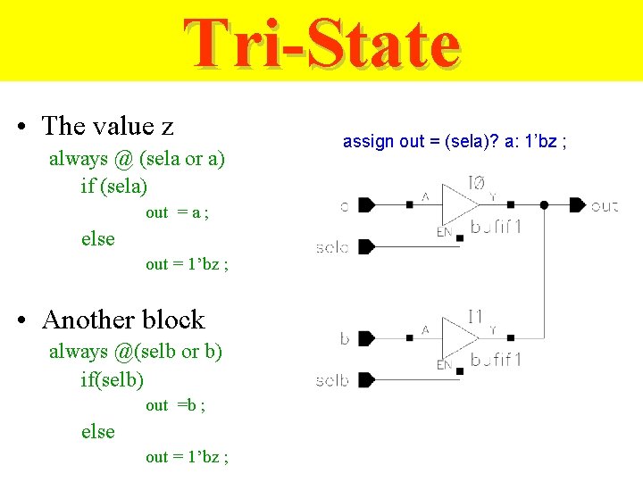
Tri-State • The value z always @ (sela or a) if (sela) out = a ; else out = 1’bz ; • Another block always @(selb or b) if(selb) out =b ; else out = 1’bz ; assign out = (sela)? a: 1’bz ;

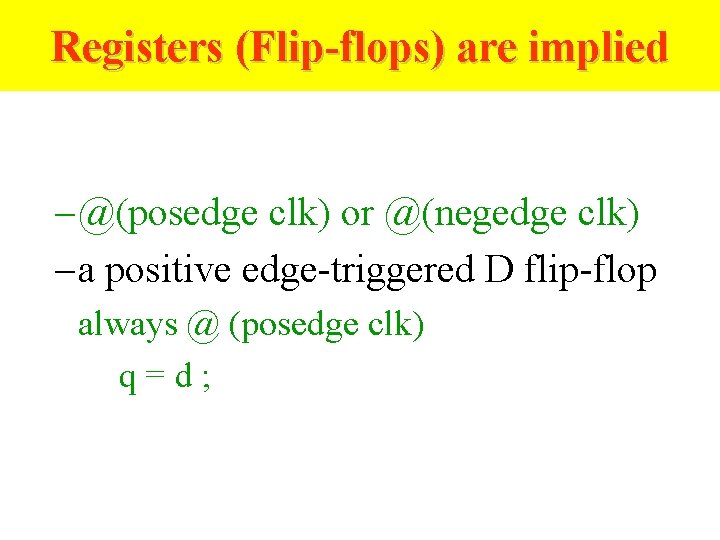
Registers (Flip-flops) are implied – @(posedge clk) or @(negedge clk) – a positive edge-triggered D flip-flop always @ (posedge clk) q=d;

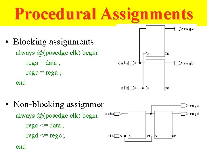
Procedural Assignments • Blocking assignments always @(posedge clk) begin rega = data ; regb = rega ; end • Non-blocking assignments always @(posedge clk) begin regc <= data ; regd <= regc ; end

Sequential Circuit Design

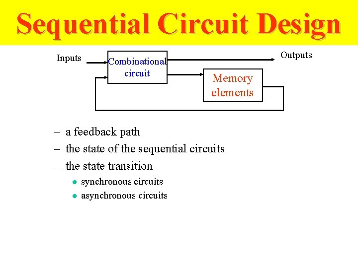
Sequential Circuit Design Inputs Combinational circuit Outputs Memory elements – a feedback path – the state of the sequential circuits – the state transition l l synchronous circuits asynchronous circuits

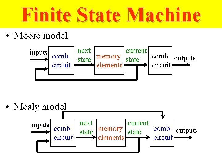
Finite State Machine • Moore model inputs comb. next memory current comb. outputs state circuit elements circuit • Mealy model inputs comb. next memory current comb. outputs state circuit elements circuit

Examples – D flip-flop – D latch – register – shifter – counter – pipeline – FSM

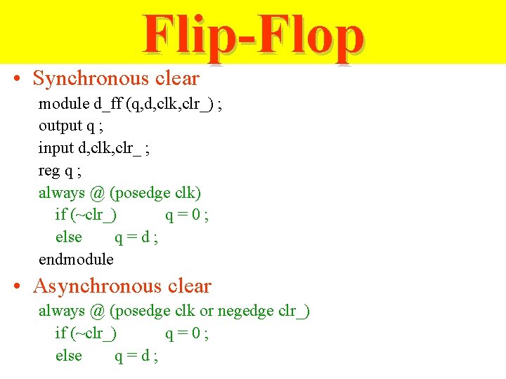
Flip-Flop • Synchronous clear module d_ff (q, d, clk, clr_) ; output q ; input d, clk, clr_ ; reg q ; always @ (posedge clk) if (~clr_) q=0; else q=d; endmodule • Asynchronous clear always @ (posedge clk or negedge clr_) if (~clr_) q=0; else q=d;

Register module register (q, d, clk, clr_, set_) ; output [7: 0] q ; input [7: 0] d ; input clk, clr_, set_ ; reg [7: 0] q ; always @ (posedge clk or negedge clr_ or negedge set_) if (~clr_) q=0; else if (~set_) q = 8’b 1111_1111 ; else q=d; endmodule

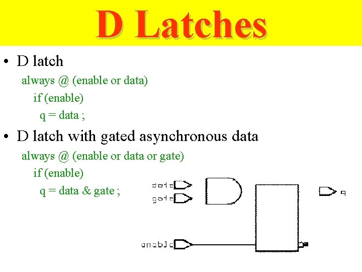
D Latches • D latch always @ (enable or data) if (enable) q = data ; • D latch with gated asynchronous data always @ (enable or data or gate) if (enable) q = data & gate ;

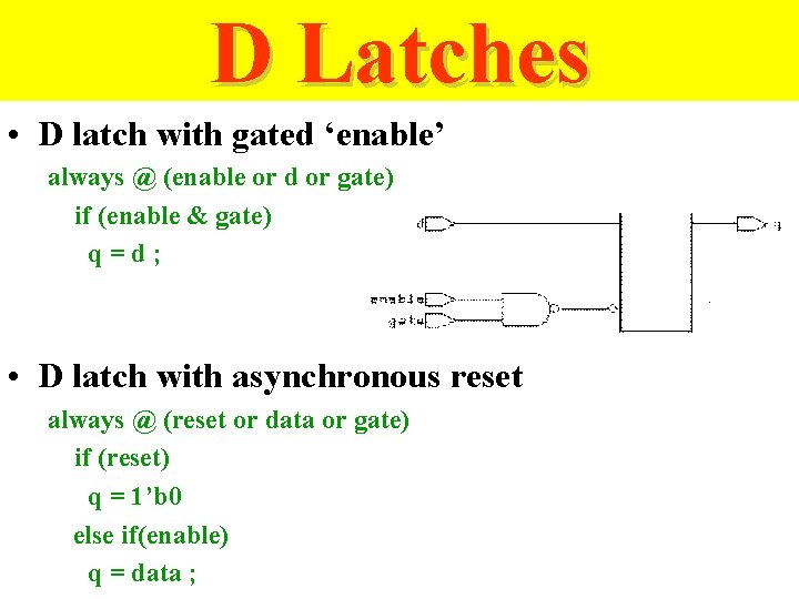
D Latches • D latch with gated ‘enable’ always @ (enable or d or gate) if (enable & gate) q=d; • D latch with asynchronous reset always @ (reset or data or gate) if (reset) q = 1’b 0 else if(enable) q = data ;

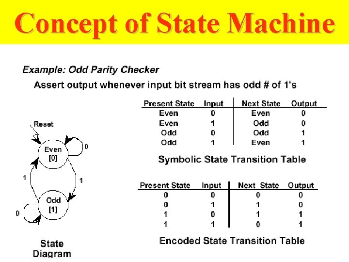
Concept of State Machine

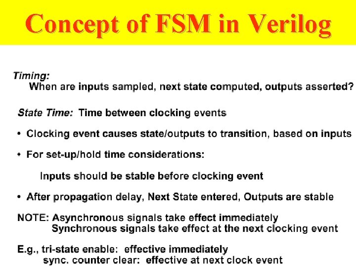
Concept of FSM in Verilog

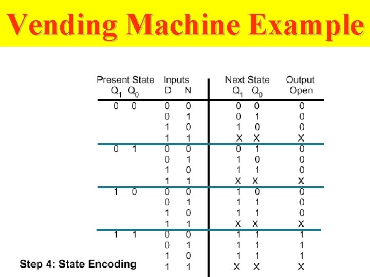
Vending Machine Example

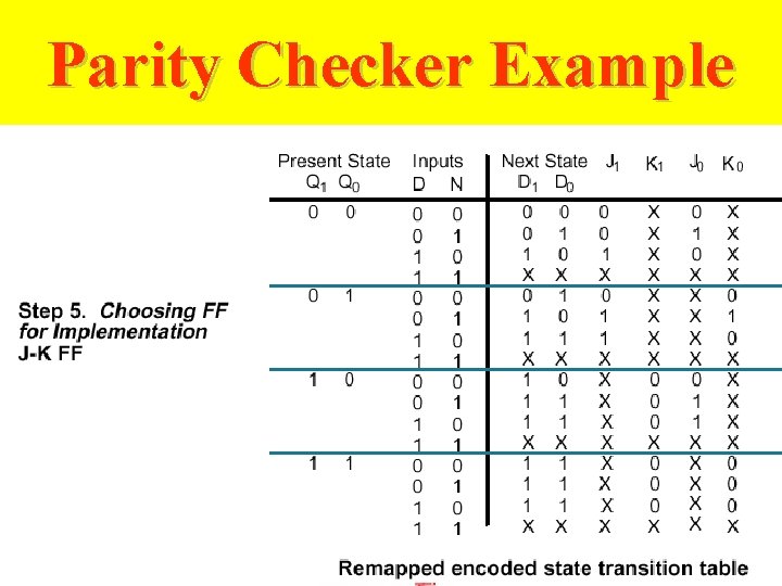
Parity Checker Example

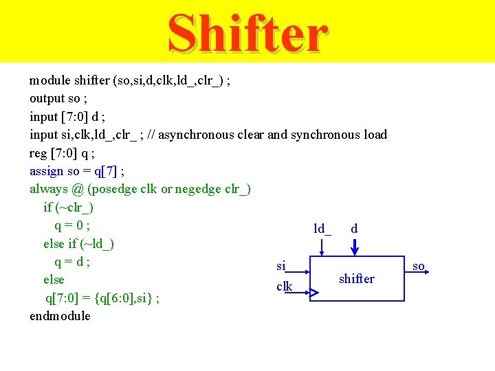
Shifter module shifter (so, si, d, clk, ld_, clr_) ; output so ; input [7: 0] d ; input si, clk, ld_, clr_ ; // asynchronous clear and synchronous load reg [7: 0] q ; assign so = q[7] ; always @ (posedge clk or negedge clr_) if (~clr_) q=0; ld_ d else if (~ld_) q=d; si shifter else clk q[7: 0] = {q[6: 0], si} ; endmodule so

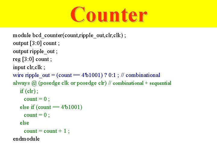
Counter module bcd_counter(count, ripple_out, clr, clk) ; output [3: 0] count ; output ripple_out ; reg [3: 0] count ; input clr, clk ; wire ripple_out = (count == 4'b 1001) ? 0: 1 ; // combinational always @ (posedge clk or posedge clr) // combinational + sequential if (clr) ; count = 0 ; else if (count == 4'b 1001) count = 0 ; else count = count + 1 ; endmodule

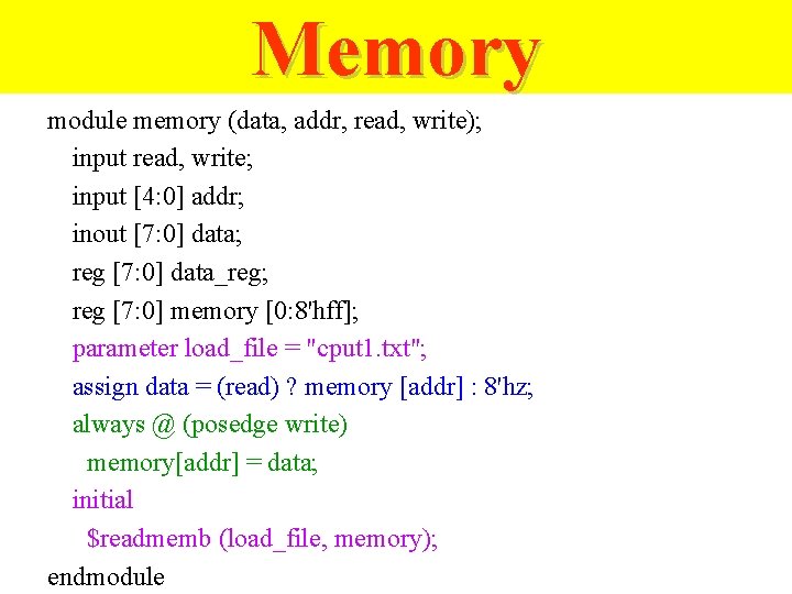
Memory module memory (data, addr, read, write); input read, write; input [4: 0] addr; inout [7: 0] data; reg [7: 0] data_reg; reg [7: 0] memory [0: 8'hff]; parameter load_file = "cput 1. txt"; assign data = (read) ? memory [addr] : 8'hz; always @ (posedge write) memory[addr] = data; initial $readmemb (load_file, memory); endmodule

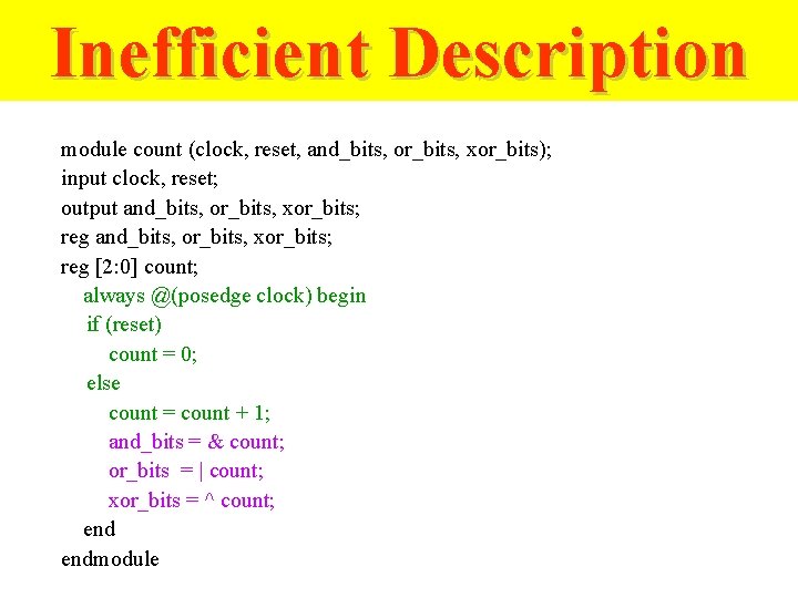
Inefficient Description module count (clock, reset, and_bits, or_bits, xor_bits); input clock, reset; output and_bits, or_bits, xor_bits; reg [2: 0] count; always @(posedge clock) begin if (reset) count = 0; else count = count + 1; and_bits = & count; or_bits = | count; xor_bits = ^ count; endmodule

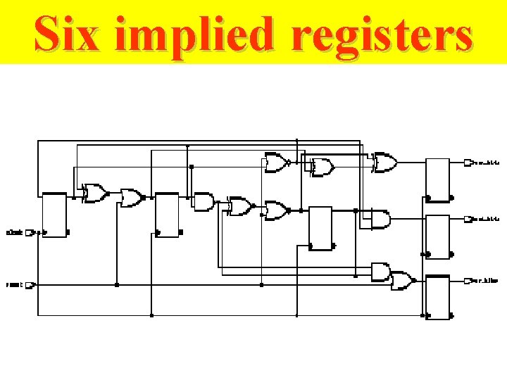
Six implied registers

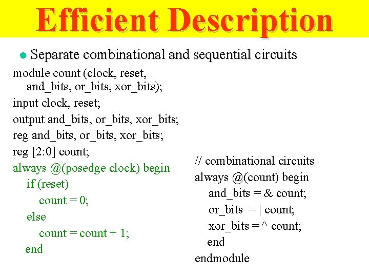
Efficient Description l Separate combinational and sequential circuits module count (clock, reset, and_bits, or_bits, xor_bits); input clock, reset; output and_bits, or_bits, xor_bits; reg [2: 0] count; always @(posedge clock) begin if (reset) count = 0; else count = count + 1; end // combinational circuits always @(count) begin and_bits = & count; or_bits = | count; xor_bits = ^ count; endmodule

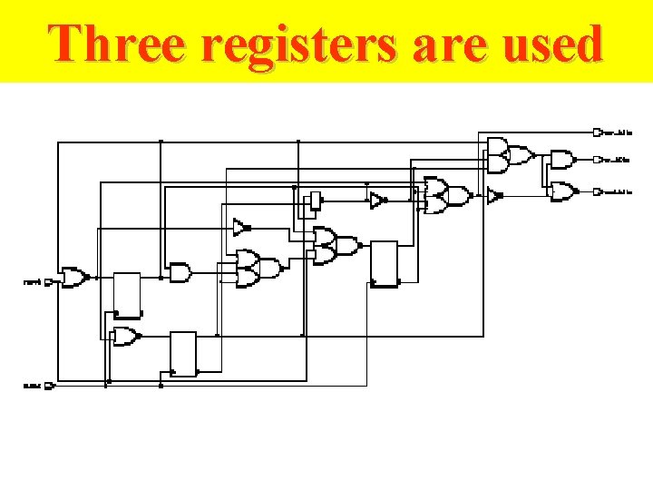
Three registers are used

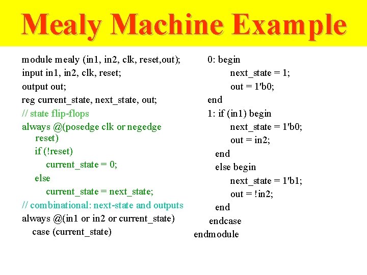
Mealy Machine Example module mealy (in 1, in 2, clk, reset, out); input in 1, in 2, clk, reset; output out; reg current_state, next_state, out; // state flip-flops always @(posedge clk or negedge reset) if (!reset) current_state = 0; else current_state = next_state; // combinational: next-state and outputs always @(in 1 or in 2 or current_state) case (current_state) 0: begin next_state = 1; out = 1'b 0; end 1: if (in 1) begin next_state = 1'b 0; out = in 2; end else begin next_state = 1'b 1; out = !in 2; endcase endmodule

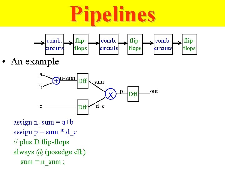
Pipelines comb. circuits flipflops comb. circuits • An example a b c n-sum Dff sum p Dff assign n_sum = a+b assign p = sum * d_c // plus D flip-flops always @ (posedge clk) sum = n_sum ; d_c Dff out flipflops

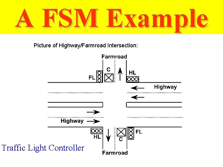
A FSM Example Picture of Highway/Farmroad Intersection: Traffic Light Controller

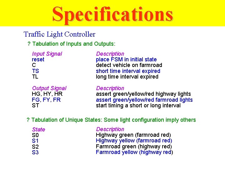
Specifications Traffic Light Controller ? Tabulation of Inputs and Outputs: Input Signal reset C TS TL Description place FSM in initial state detect vehicle on farmroad short time interval expired long time interval expired Output Signal HG, HY, HR FG, FY, FR ST Description assert green/yellow/red highway lights assert green/yellow/red farmroad lights start timing a short or long interval ? Tabulation of Unique States: Some light configuration imply others State S 0 S 1 S 2 S 3 Description Highway green (farmroad red) Highway yellow (farmroad red) Farmroad green (highway red) Farmroad yellow (highway red)

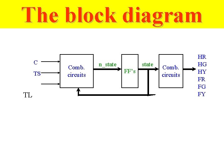
The block diagram C TS TL Comb. circuits n_state FF’s Comb. circuits HR HG HY FR FG FY

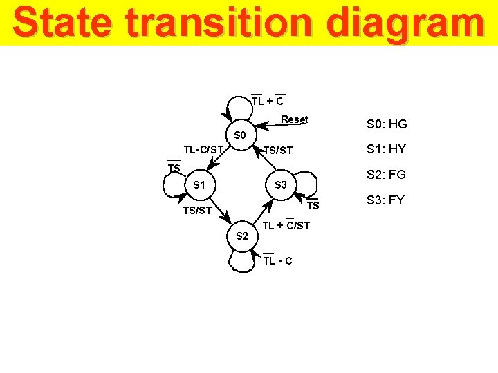
State transition diagram TL + C Reset S 0 TL • C/ST S 1: HY TS/ST TS S 1 S 2: FG S 3 TS TS/ST S 2 TL + C/ST TL • C S 0: HG S 3: FY

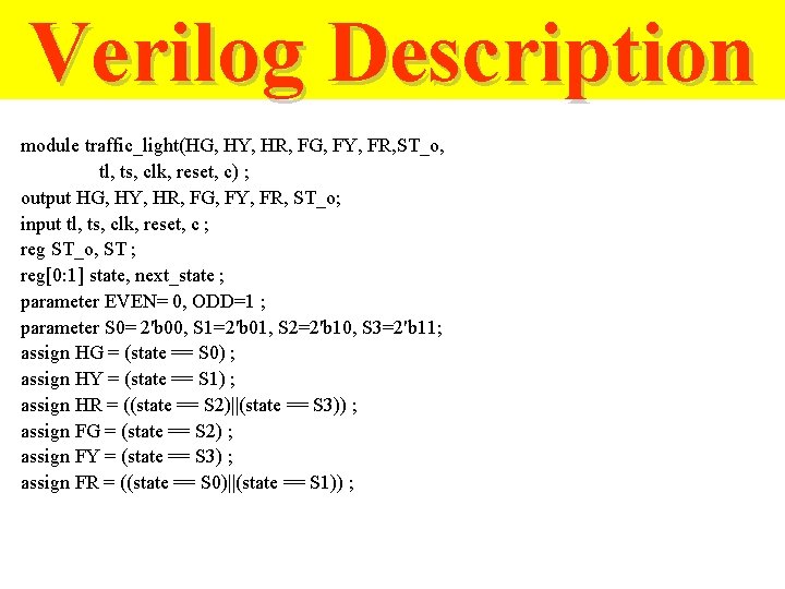
Verilog Description module traffic_light(HG, HY, HR, FG, FY, FR, ST_o, tl, ts, clk, reset, c) ; output HG, HY, HR, FG, FY, FR, ST_o; input tl, ts, clk, reset, c ; reg ST_o, ST ; reg[0: 1] state, next_state ; parameter EVEN= 0, ODD=1 ; parameter S 0= 2'b 00, S 1=2'b 01, S 2=2'b 10, S 3=2'b 11; assign HG = (state == S 0) ; assign HY = (state == S 1) ; assign HR = ((state == S 2)||(state == S 3)) ; assign FG = (state == S 2) ; assign FY = (state == S 3) ; assign FR = ((state == S 0)||(state == S 1)) ;

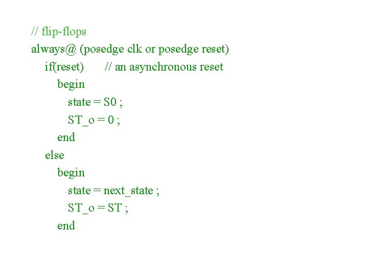
// flip-flops always@ (posedge clk or posedge reset) if(reset) // an asynchronous reset begin state = S 0 ; ST_o = 0 ; end else begin state = next_state ; ST_o = ST ; end

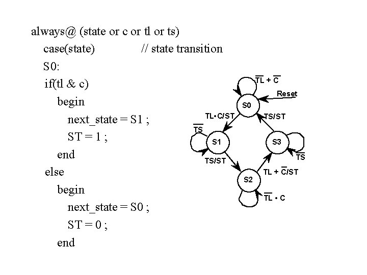
always@ (state or c or tl or ts) case(state) // state transition S 0: if(tl & c) begin TL • C/ST next_state = S 1 ; TS ST = 1 ; S 1 end TS/ST else begin next_state = S 0 ; ST = 0 ; end TL + C Reset S 0 TS/ST S 3 TS S 2 TL + C/ST TL • C

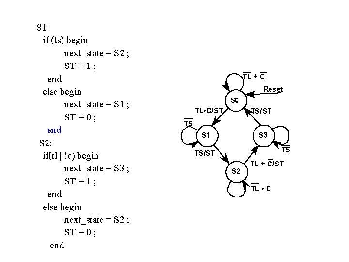
S 1: if (ts) begin next_state = S 2 ; ST = 1 ; end else begin next_state = S 1 ; ST = 0 ; end S 2: if(tl | !c) begin next_state = S 3 ; ST = 1 ; end else begin next_state = S 2 ; ST = 0 ; end TL + C Reset S 0 TL • C/ST TS S 1 S 3 TS TS/ST S 2 TL + C/ST TL • C

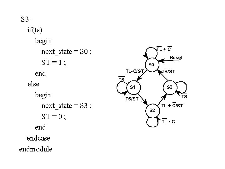
S 3: if(ts) begin next_state = S 0 ; ST = 1 ; end else begin next_state = S 3 ; ST = 0 ; endcase endmodule TL + C Reset S 0 TL • C/ST TS S 1 S 3 TS TS/ST S 2 TL + C/ST TL • C

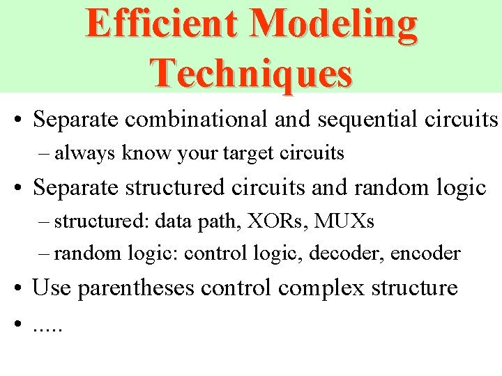
Efficient Modeling Techniques • Separate combinational and sequential circuits – always know your target circuits • Separate structured circuits and random logic – structured: data path, XORs, MUXs – random logic: control logic, decoder, encoder • Use parentheses control complex structure • . . .

VERILOG Coding Styles Synthesizable Behavioral Register Transfer Level (RTL) Structural

Behavioral modeling

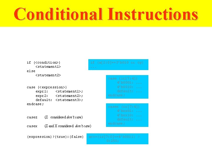
Conditional Instructions if (<condition>) <statement 1> else <statement 2> if (a[2: 0]==3’b 010 && cy). . . case (ir[7: 4]) 4’b 0001: . . . 4’b 0010: . . . default: . . . endcase; case (<expression>) expr 1: <statement 1>; expr 2: <statement 2>; default: <statement 3>; endcase; casez (Z considered don’t care) casex (Z and X considered don’t care) (expression)? (true): (false) casex (ir[7: 4]) 4’bxx 01: . . . 4’bxx 10: . . . default: . . . endcase; acc=(ir[7: 0]==4’b 0011) ? 0: 255;

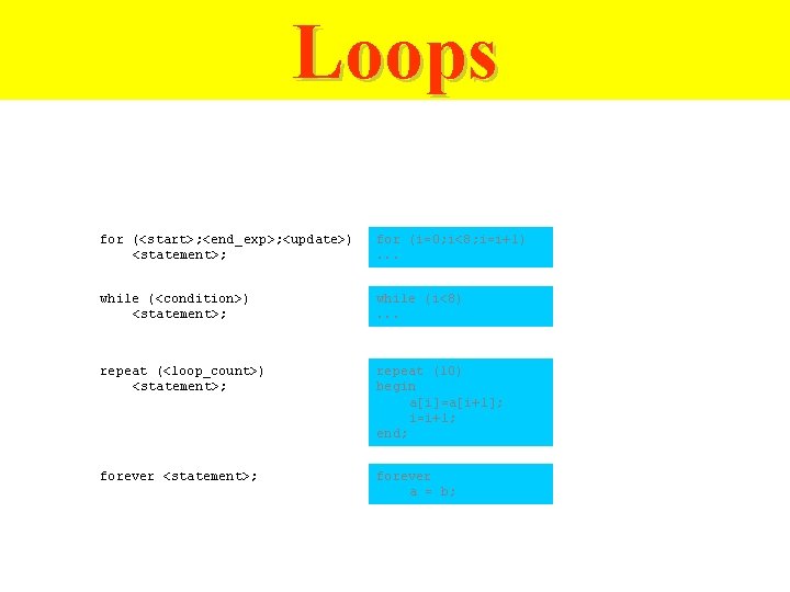
Loops for (<start>; <end_exp>; <update>) <statement>; for (i=0; i<8; i=i+1). . . while (<condition>) <statement>; while (i<8). . . repeat (<loop_count>) <statement>; repeat (10) begin a[i]=a[i+1]; i=i+1; end; forever <statement>; forever a = b;

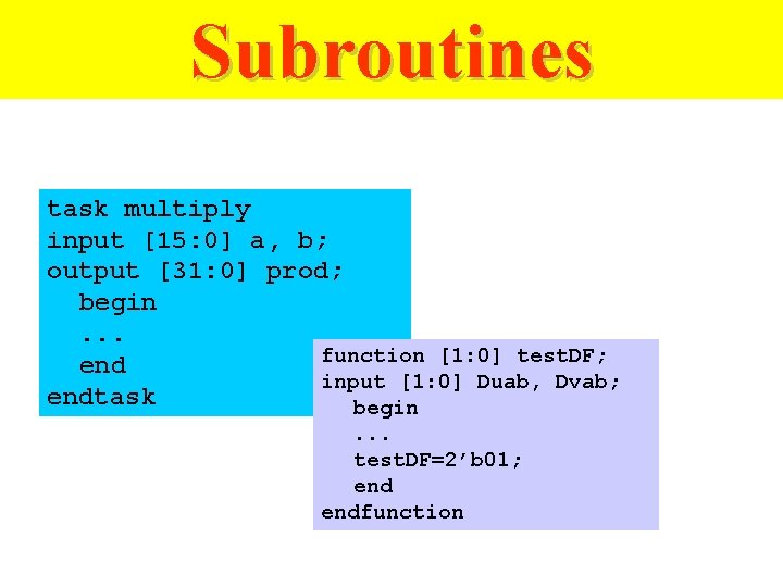
Subroutines task multiply input [15: 0] a, b; output [31: 0] prod; begin. . . function [1: 0] test. DF; end input [1: 0] Duab, Dvab; endtask begin. . . test. DF=2’b 01; endfunction

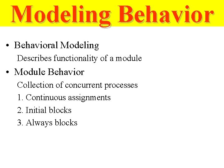
Modeling Behavior • Behavioral Modeling Describes functionality of a module • Module Behavior Collection of concurrent processes 1. Continuous assignments 2. Initial blocks 3. Always blocks

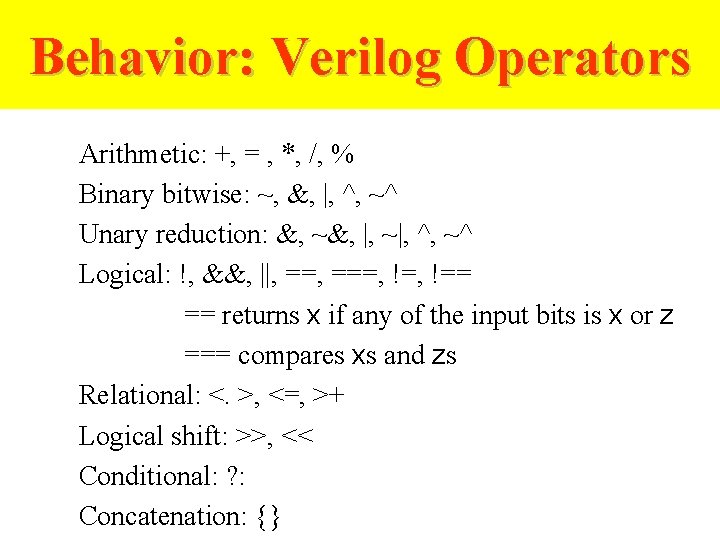
Behavior: Verilog Operators Arithmetic: +, = , *, /, % Binary bitwise: ~, &, |, ^, ~^ Unary reduction: &, ~&, |, ~|, ^, ~^ Logical: !, &&, ||, ===, !== == returns x if any of the input bits is x or z === compares xs and zs Relational: <. >, <=, >+ Logical shift: >>, << Conditional: ? : Concatenation: {}

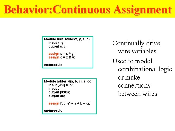
Behavior: Continuous Assignment Module half_adder(x, y, s, c) input x, y; output s, c; assign s = x ^ y; assign c = x & y; endmodule Module adder_4(a, b, ci, s, co) input [3: 0] a, b; input ci; output [3: 0]s; output co; assign {co, s} = a + b + ci; endmodule Continually drive wire variables Used to model combinational logic or make connections between wires

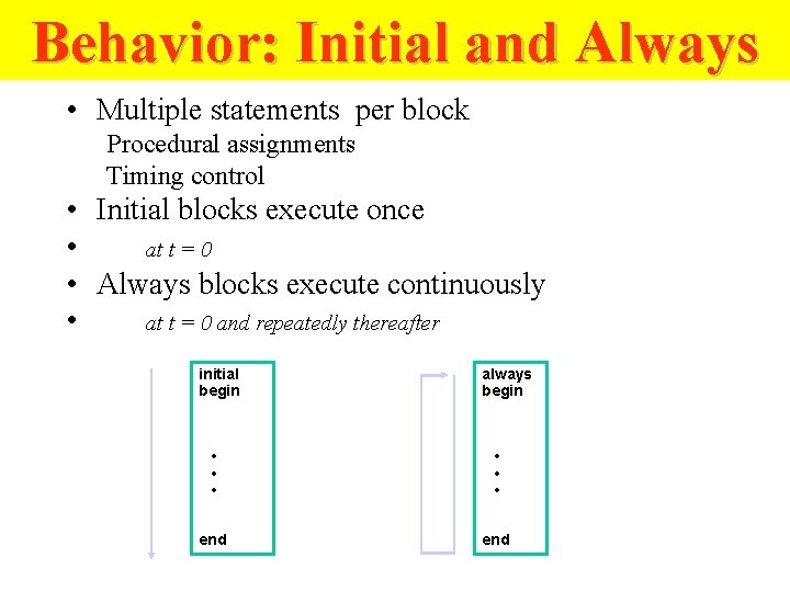
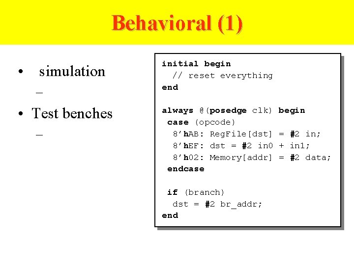
Behavior: Initial and Always • Multiple statements per block Procedural assignments Timing control • Initial blocks execute once • at t = 0 • Always blocks execute continuously • at t = 0 and repeatedly thereafter initial begin always begin • • • end

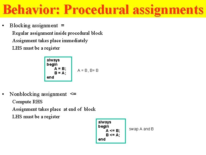
Behavior: Procedural assignments • Blocking assignment = Regular assignment inside procedural block Assignment takes place immediately LHS must be a register always begin A = B; B = A; end A = B, B= B • Nonblocking assignment <= Compute RHS Assignment takes place at end of block LHS must be a register always begin A <= B; B <= A; end swap A and B

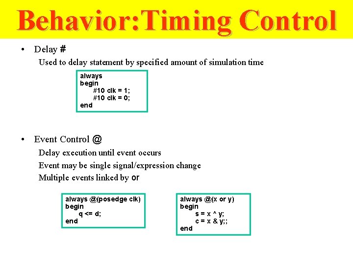
Behavior: Timing Control • Delay # Used to delay statement by specified amount of simulation time always begin #10 clk = 1; #10 clk = 0; end • Event Control @ Delay execution until event occurs Event may be single signal/expression change Multiple events linked by or always @(posedge clk) begin q <= d; end always @(x or y) begin s = x ^ y; c = x & y; ; end

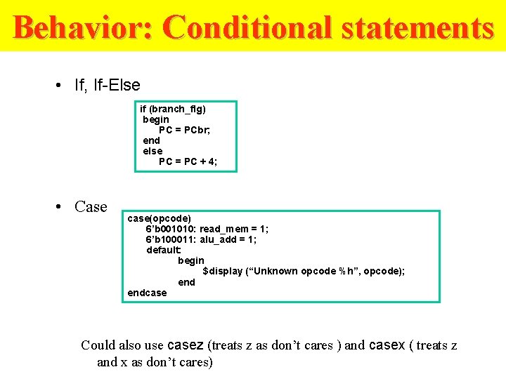
Behavior: Conditional statements • If, If-Else if (branch_flg) begin PC = PCbr; end else PC = PC + 4; • Case case(opcode) 6’b 001010: read_mem = 1; 6’b 100011: alu_add = 1; default: begin $display (“Unknown opcode %h”, opcode); endcase Could also use casez (treats z as don’t cares ) and casex ( treats z and x as don’t cares)

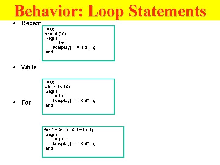
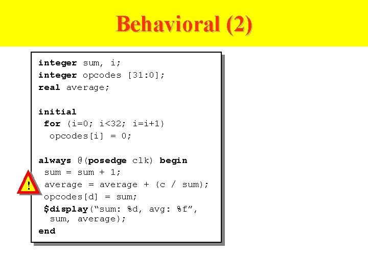
Behavior: Loop Statements • Repeat i = 0; repeat (10) begin i = i + 1; $display( “i = %d”, i); end • While • For i = 0; while (i < 10) begin i = i + 1; $display( “i = %d”, i); end for (i = 0; i < 10; i = i + 1) begin i = i + 1; $display( “i = %d”, i); end

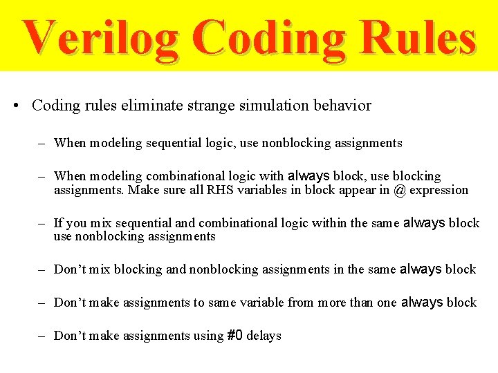
Verilog Coding Rules • Coding rules eliminate strange simulation behavior – When modeling sequential logic, use nonblocking assignments – When modeling combinational logic with always block, use blocking assignments. Make sure all RHS variables in block appear in @ expression – If you mix sequential and combinational logic within the same always block use nonblocking assignments – Don’t mix blocking and nonblocking assignments in the same always block – Don’t make assignments to same variable from more than one always block – Don’t make assignments using #0 delays

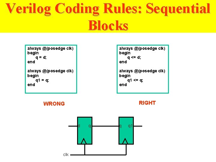
Verilog Coding Rules: Sequential Blocks always @(posedge clk) begin q = d; end always @(posedge clk) begin q <= d; end always @(posedge clk) begin q 1 = q; end always @(posedge clk) begin q 1 <= q; end RIGHT WRONG d clk q q q 1

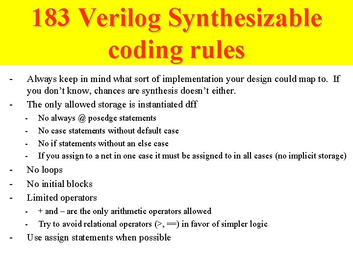
183 Verilog Synthesizable coding rules - Always keep in mind what sort of implementation your design could map to. If you don’t know, chances are synthesis doesn’t either. The only allowed storage is instantiated dff - - No loops No initial blocks Limited operators - - No always @ posedge statements No case statements without default case No if statements without an else case If you assign to a net in one case it must be assigned to in all cases (no implicit storage) + and – are the only arithmetic operators allowed Try to avoid relational operators (>, ==) in favor of simpler logic Use assign statements when possible

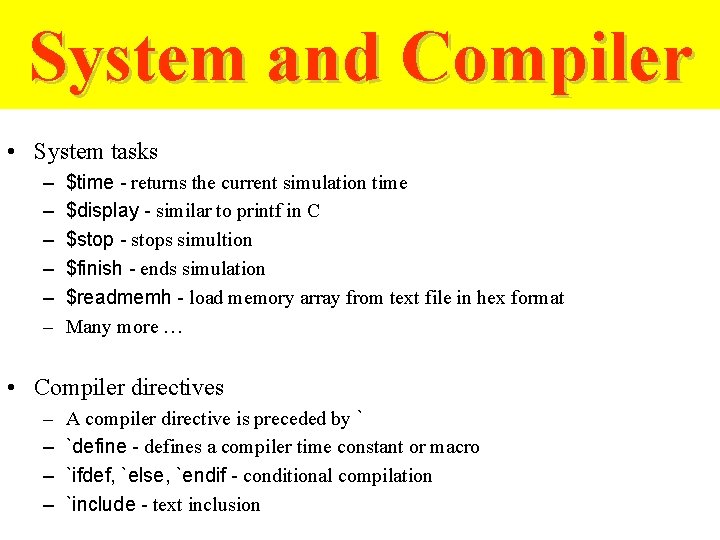
System and Compiler • System tasks – – – $time - returns the current simulation time $display - similar to printf in C $stop - stops simultion $finish - ends simulation $readmemh - load memory array from text file in hex format Many more … • Compiler directives – – A compiler directive is preceded by ` `define - defines a compiler time constant or macro `ifdef, `else, `endif - conditional compilation `include - text inclusion

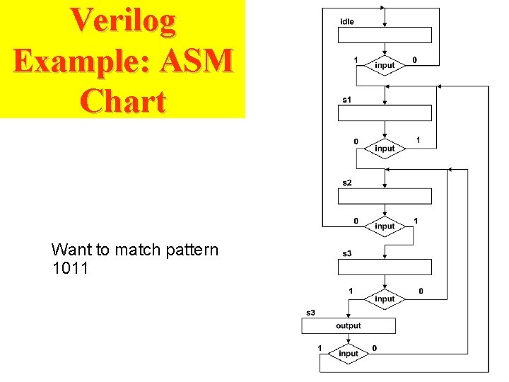
Verilog Example: ASM Chart Want to match pattern 1011

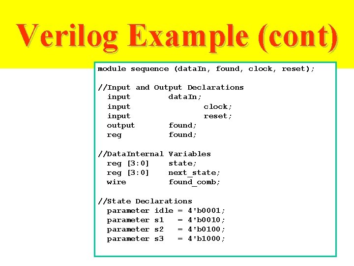
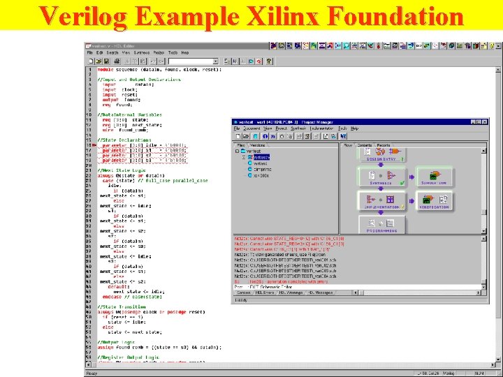
Verilog Example (cont) module sequence (data. In, found, clock, reset); //Input and Output Declarations input data. In; input clock; input reset; output found; reg found; //Data. Internal reg [3: 0] wire Variables state; next_state; found_comb; //State Declarations parameter idle = 4'b 0001; parameter s 1 = 4'b 0010; parameter s 2 = 4'b 0100; parameter s 3 = 4'b 1000;

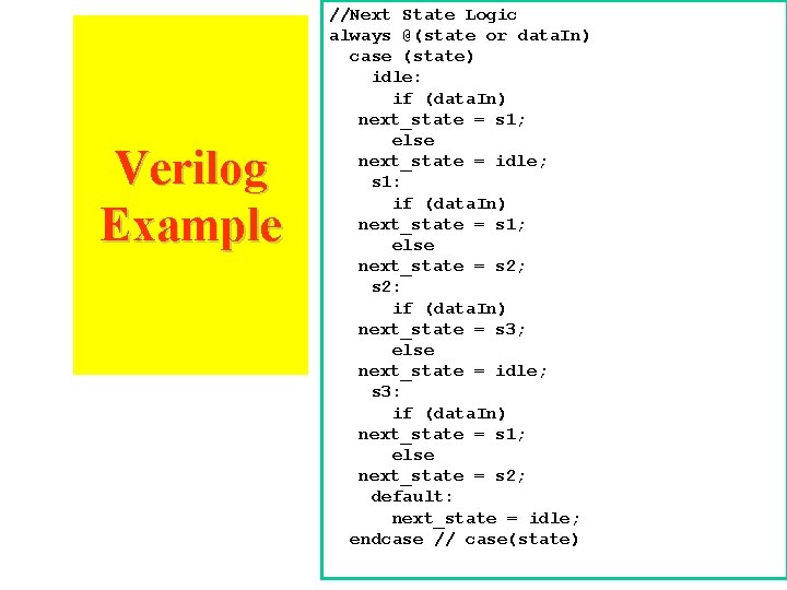
Verilog Example //Next State Logic always @(state or data. In) case (state) idle: if (data. In) next_state = s 1; else next_state = idle; s 1: if (data. In) next_state = s 1; else next_state = s 2; s 2: if (data. In) next_state = s 3; else next_state = idle; s 3: if (data. In) next_state = s 1; else next_state = s 2; default: next_state = idle; endcase // case(state)

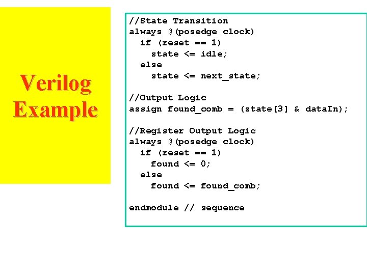
Verilog Example //State Transition always @(posedge clock) if (reset == 1) state <= idle; else state <= next_state; //Output Logic assign found_comb = (state[3] & data. In); //Register Output Logic always @(posedge clock) if (reset == 1) found <= 0; else found <= found_comb; endmodule // sequence

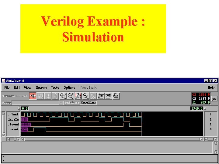
Verilog Example : Simulation

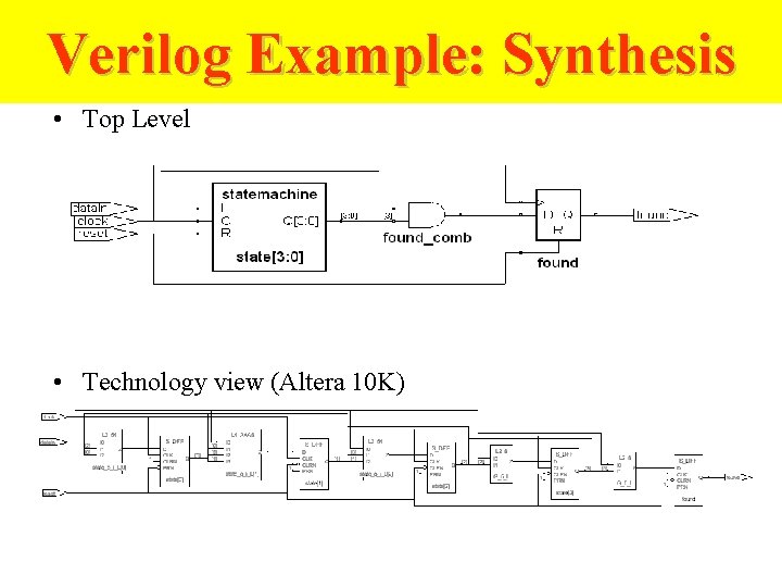
Verilog Example: Synthesis • Top Level • Technology view (Altera 10 K)

Verilog Example Xilinx Foundation

Verilog Example Xilinx Foundation

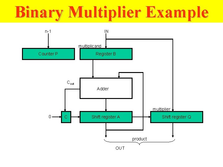
Binary Multiplier Example n-1 IN multiplicand Counter P Register B Cout Adder multiplier 0 C Shift register A Shift register Q product OUT

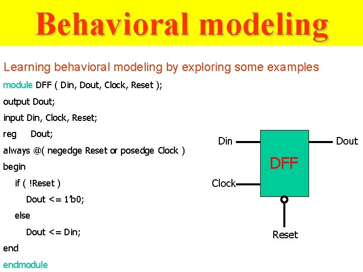
Behavioral modeling Learning behavioral modeling by exploring some examples module DFF ( Din, Dout, Clock, Reset ); output Dout; input Din, Clock, Reset; reg Dout; always @( negedge Reset or posedge Clock ) Din DFF begin if ( !Reset ) Dout Clock Dout <= 1’b 0; else Dout <= Din; endmodule Reset

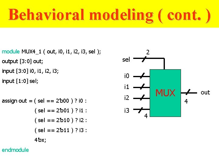
Behavioral modeling ( cont. ) module MUX 4_1 ( out, i 0, i 1, i 2, i 3, sel ); output [3: 0] out; input [3: 0] i 0, i 1, i 2, i 3; input [1: 0] sel; sel i 0 i 1 assign out = ( sel == 2’b 00 ) ? i 0 : i 2 ( sel == 2’b 01 ) ? i 1 : i 3 ( sel == 2’b 10 ) ? i 2 : ( sel == 2’b 11 ) ? i 3 : 4’bx; endmodule 2 MUX 4 out 4

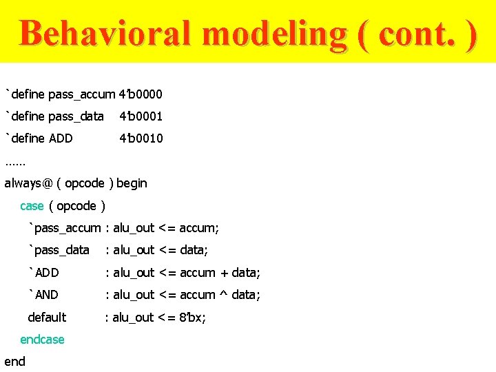
Behavioral modeling ( cont. ) `define pass_accum 4’b 0000 `define pass_data 4’b 0001 `define ADD 4’b 0010 …… always@ ( opcode ) begin case ( opcode ) `pass_accum : alu_out <= accum; `pass_data : alu_out <= data; `ADD : alu_out <= accum + data; `AND : alu_out <= accum ^ data; default : alu_out <= 8’bx; endcase end

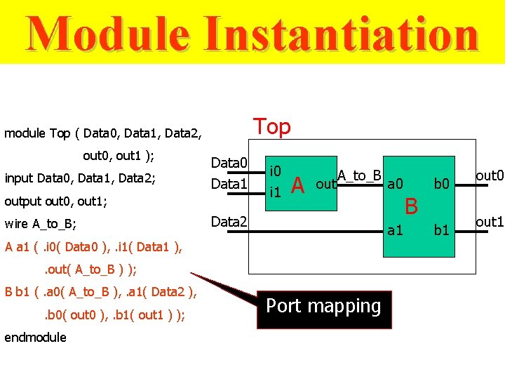
Module Instantiation Top module Top ( Data 0, Data 1, Data 2, out 0, out 1 ); input Data 0, Data 1, Data 2; Data 0 Data 1 output out 0, out 1; wire A_to_B; i 0 i 1 A out A_to_B Data 2 a 1 A a 1 (. i 0( Data 0 ), . i 1( Data 1 ), . out( A_to_B ) ); B b 1 (. a 0( A_to_B ), . a 1( Data 2 ), . b 0( out 0 ), . b 1( out 1 ) ); endmodule a 0 Port mapping B b 0 b 1 out 0 out 1

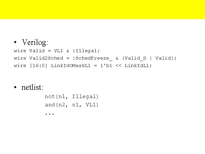
• Verilog: wire Valid = VL 1 & !Illegal; wire Valid 2 Sched = !Sched. Freeze_ & (Valid_D | Valid); wire [16: 0] Link. Id. OMask. L 1 = 1'b 1 << Link. Id. L 1; • netlist: not(n 1, Illegal) and(n 2, n 1, VL 1). . .

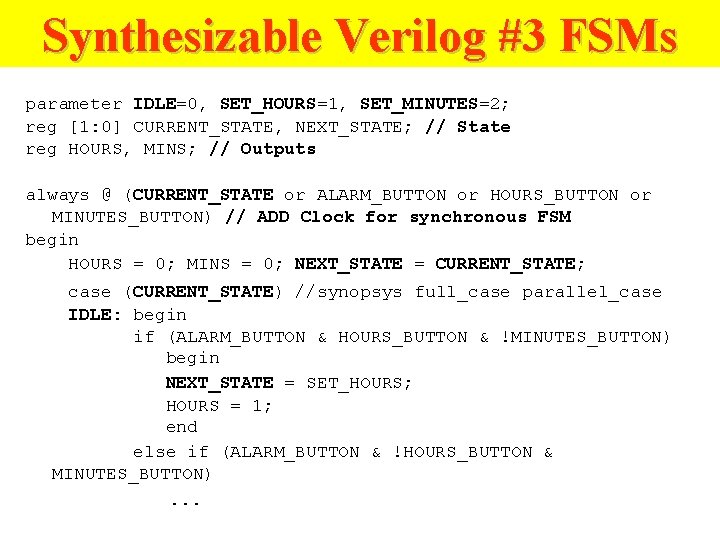
Synthesizable Verilog #3 FSMs parameter IDLE=0, SET_HOURS=1, SET_MINUTES=2; reg [1: 0] CURRENT_STATE, NEXT_STATE; // State reg HOURS, MINS; // Outputs always @ (CURRENT_STATE or ALARM_BUTTON or HOURS_BUTTON or MINUTES_BUTTON) // ADD Clock for synchronous FSM begin HOURS = 0; MINS = 0; NEXT_STATE = CURRENT_STATE; case (CURRENT_STATE) //synopsys full_case parallel_case IDLE: begin if (ALARM_BUTTON & HOURS_BUTTON & !MINUTES_BUTTON) begin NEXT_STATE = SET_HOURS; HOURS = 1; end else if (ALARM_BUTTON & !HOURS_BUTTON & MINUTES_BUTTON). . .

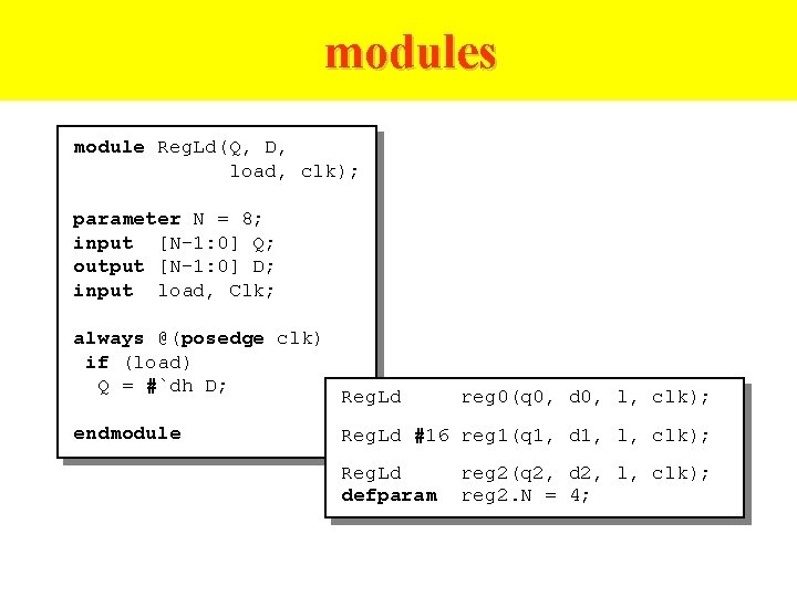
modules module Reg. Ld(Q, D, load, clk); parameter N = 8; input [N-1: 0] Q; output [N-1: 0] D; input load, Clk; always @(posedge clk) if (load) Q = #`dh D; endmodule Reg. Ld reg 0(q 0, d 0, l, clk); Reg. Ld #16 reg 1(q 1, d 1, l, clk); Reg. Ld defparam reg 2(q 2, d 2, l, clk); reg 2. N = 4;

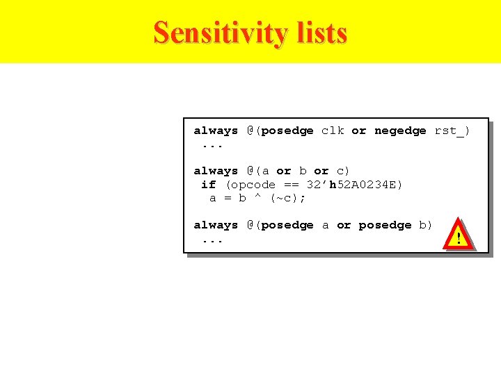
Sensitivity lists always @(posedge clk or negedge rst_). . . always @(a or b or c) if (opcode == 32’h 52 A 0234 E) a = b ^ (~c); always @(posedge a or posedge b). . . !

Behavioral (1) • simulation – • Test benches – initial begin // reset everything end always @(posedge clk) case (opcode) 8’h. AB: Reg. File[dst] 8’h. EF: dst = #2 in 0 8’h 02: Memory[addr] endcase if (branch) dst = #2 br_addr; end begin = #2 in; + in 1; = #2 data;

Behavioral (2) integer sum, i; integer opcodes [31: 0]; real average; initial for (i=0; i<32; i=i+1) opcodes[i] = 0; ! always @(posedge clk) begin sum = sum + 1; average = average + (c / sum); opcodes[d] = sum; $display(“sum: %d, avg: %f”, sum, average); end

Verification of Design

Differences between Tasks and Functions

Tasks versus Functions in Verilog • Procedures/Subroutines/Functions in SW programming languages – The same functionality, in different places • Verilog equivalence: – Tasks and Functions – Used in behavioral modeling – Part of design hierarchy Hierarchical name

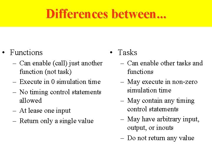
Differences between. . . • Functions – Can enable (call) just another function (not task) – Execute in 0 simulation time – No timing control statements allowed – At lease one input – Return only a single value • Tasks – Can enable other tasks and functions – May execute in non-zero simulation time – May contain any timing control statements – May have arbitrary input, output, or inouts – Do not return any value

Differences between… (cont’d) • Both – – – are defined in a module are local to the module can have local variables (registers, but not nets) and events contain only behavioral statements do not contain initial or always statements are called from initial or always statements or other tasks or functions

Differences between… (cont’d) • Tasks can be used for common Verilog code • Function are used when the common code – is purely combinational – executes in 0 simulation time – provides exactly one output • Functions are typically used for conversions and commonly used calculations

Tasks

Tasks • Keywords: task, endtask • Must be used if the procedure has – any timing control constructs – zero or more than one output arguments – no input arguments

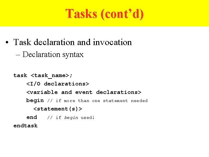
Tasks (cont’d) • Task declaration and invocation – Declaration syntax task <task_name>; <I/O declarations> <variable and event declarations> begin // if more than one statement needed <statement(s)> end // if begin used! endtask

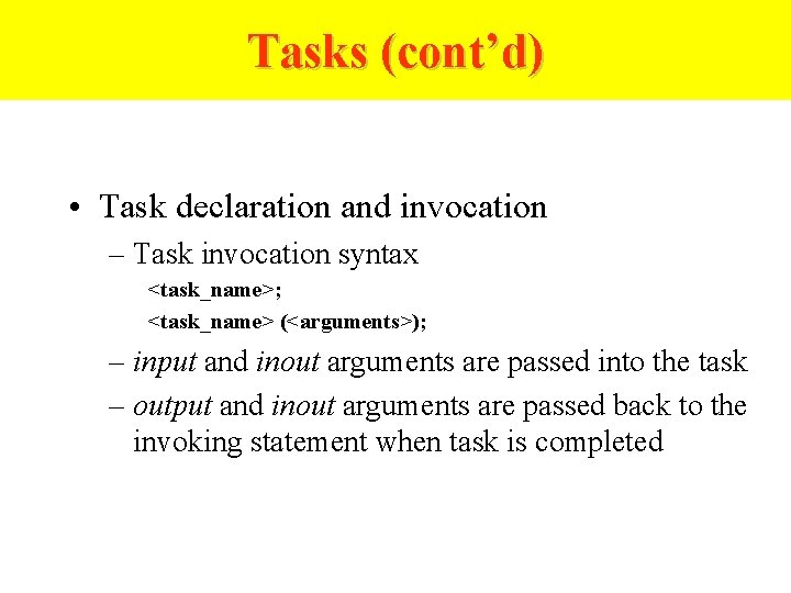
Tasks (cont’d) • Task declaration and invocation – Task invocation syntax <task_name>; <task_name> (<arguments>); – input and inout arguments are passed into the task – output and inout arguments are passed back to the invoking statement when task is completed

Tasks (cont’d) • I/O declaration in modules vs. tasks – Both used keywords: input, output, inout – In modules, represent ports • connect to external signals – In tasks, represent arguments • pass values to and from the task

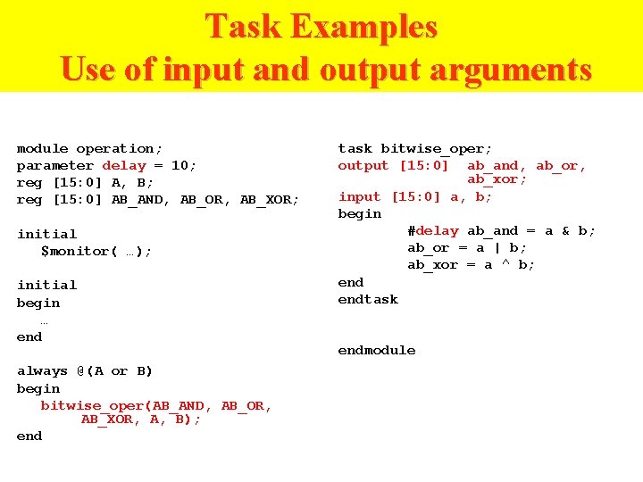
Task Examples Use of input and output arguments module operation; parameter delay = 10; reg [15: 0] A, B; reg [15: 0] AB_AND, AB_OR, AB_XOR; initial $monitor( …); initial begin … end always @(A or B) begin bitwise_oper(AB_AND, AB_OR, AB_XOR, A, B); end task bitwise_oper; output [15: 0] ab_and, ab_or, ab_xor; input [15: 0] a, b; begin #delay ab_and = a & b; ab_or = a | b; ab_xor = a ^ b; endtask endmodule

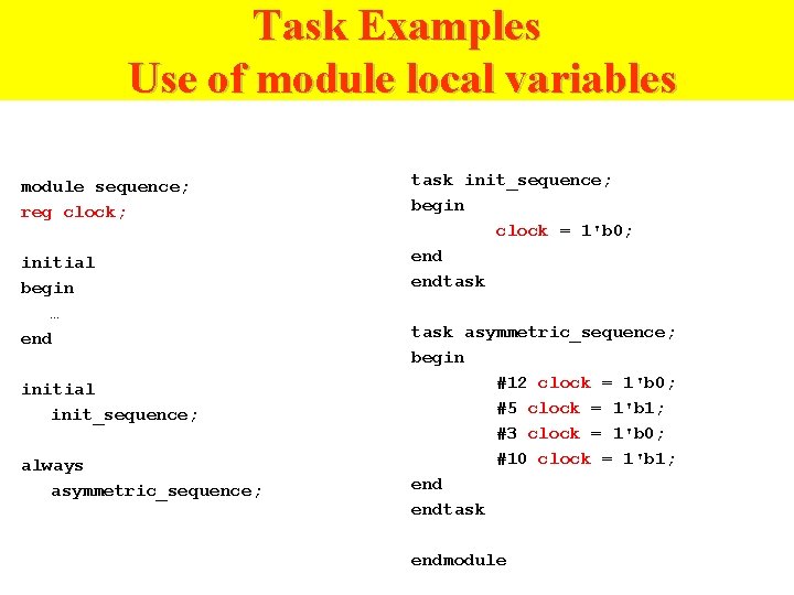
Task Examples Use of module local variables module sequence; reg clock; initial begin … end initial init_sequence; always asymmetric_sequence; task init_sequence; begin clock = 1'b 0; endtask asymmetric_sequence; begin #12 clock = 1'b 0; #5 clock = 1'b 1; #3 clock = 1'b 0; #10 clock = 1'b 1; endtask endmodule

Functions

Functions • Keyword: function, endfunction • Can be used if the procedure – does not have any timing control constructs – returns exactly a single value – has at least one input argument

Functions (cont’d) • Function Declaration and Invocation – Declaration syntax: function <range_or_type> <func_name>; <input declaration(s)> <variable_declaration(s)> begin // if more than one statement needed <statements> end // if begin used endfunction

Functions (cont’d) • Function Declaration and Invocation – Invocation syntax: <func_name> (<argument(s)>);

Functions (cont’d) • Semantics – much like function in Pascal – An internal implicit reg is declared inside the function with the same name – The return value is specified by setting that implicit reg – <range_or_type> defines width and type of the implicit reg • type can be integer or real • default bit width is 1

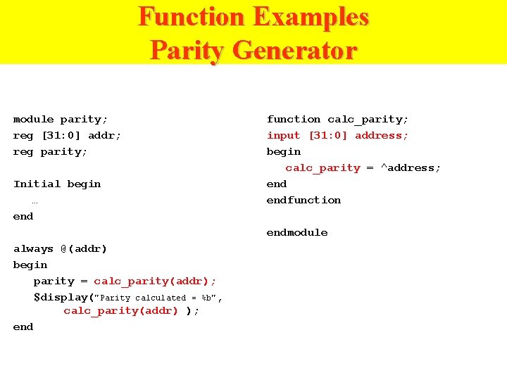
Function Examples Parity Generator module parity; reg [31: 0] addr; reg parity; Initial begin … end function calc_parity; input [31: 0] address; begin calc_parity = ^address; endfunction endmodule always @(addr) begin parity = calc_parity(addr); $display("Parity calculated = %b" , calc_parity(addr) ); end

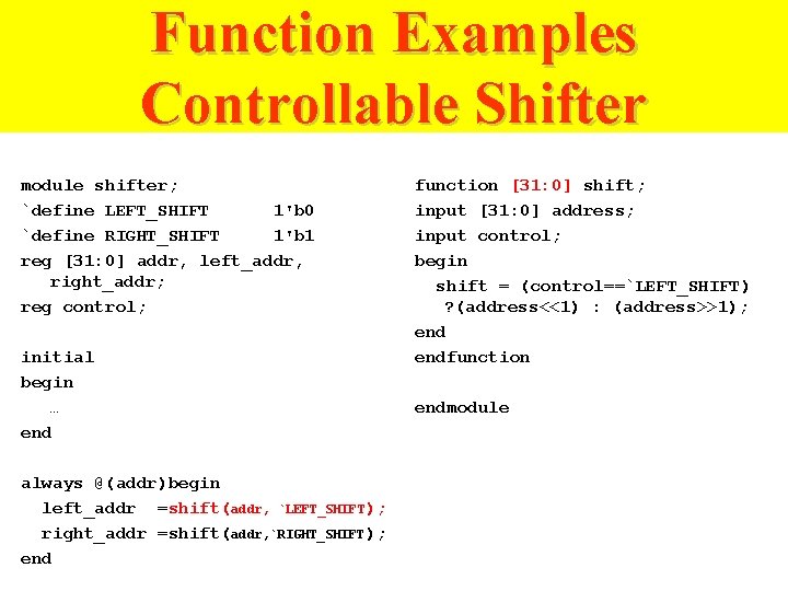
Function Examples Controllable Shifter module shifter; `define LEFT_SHIFT 1'b 0 `define RIGHT_SHIFT 1'b 1 reg [31: 0] addr, left_addr, right_addr; reg control; initial begin … end always @(addr)begin left_addr =shift(addr, `LEFT_SHIFT ); right_addr =shift(addr, `RIGHT_SHIFT ); end function [31: 0] shift; input [31: 0] address; input control; begin shift = (control==`LEFT_SHIFT) ? (address<<1) : (address>>1); endfunction endmodule

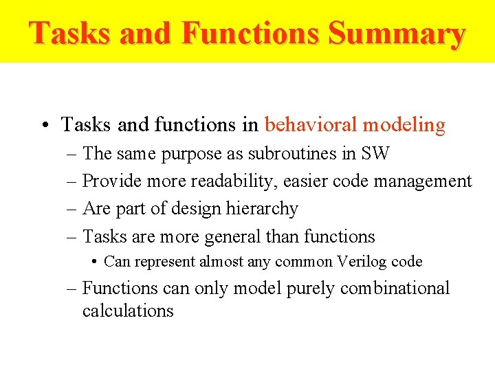
Tasks and Functions Summary • Tasks and functions in behavioral modeling – The same purpose as subroutines in SW – Provide more readability, easier code management – Are part of design hierarchy – Tasks are more general than functions • Can represent almost any common Verilog code – Functions can only model purely combinational calculations

Chap 5. Arithmetic Functions and Circuits Spring 2004 Jong Won Park jwpark@crow. cnu. ac. kr

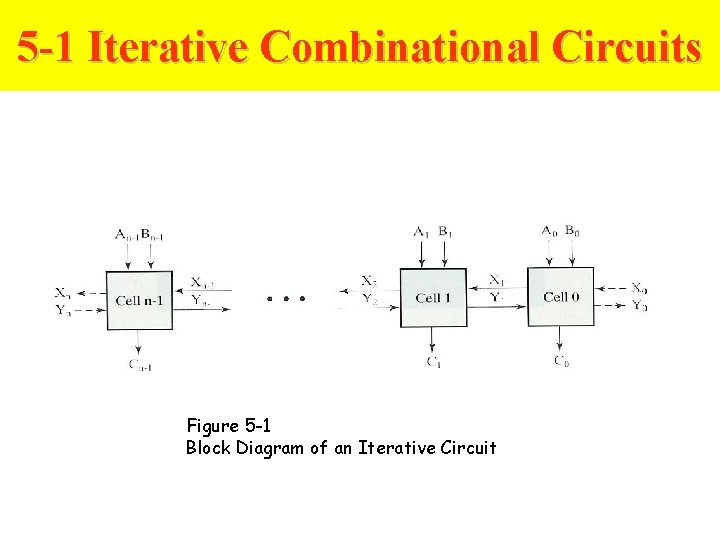
5 -1 Iterative Combinational Circuits Figure 5 -1 Block Diagram of an Iterative Circuit

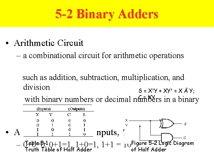
5 -2 Binary Adders • Arithmetic Circuit – a combinational circuit for arithmetic operations such as addition, subtraction, multiplication, and division S = X'Y + XY' = X Å Y; C = XY with binary numbers or decimal numbers in a binary code • Addition of 2 binary inputs, 'Half Adder‘ Table 5 -1 0+1=1, 1+0=1, 1+1 = 10 Figure 5 -2 Logic Diagram – 0+0=0, Truth Table of Half Adder

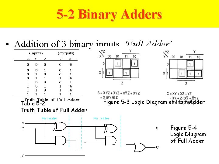
5 -2 Binary Adders • Addition of 3 binary inputs, 'Full Adder' Table 5 -2 Truth Table of Full Adder Figure 5 -3 Logic Diagram of Half Adder Figure 5 -4 Logic Diagram of Full Adder

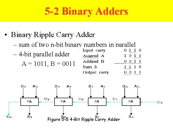
5 -2 Binary Adders • Binary Ripple Carry Adder – sum of two n-bit binary numbers in parallel – 4 -bit parallel adder A = 1011, B = 0011 Figure 5 -5 4 -Bit Ripple Carry Adder

5 -2 Binary Adders • Carry Lookahead Adder – The ripple carry adder has a long circuit delay • the longest delay: 2 n + 2 gate delay Carry Lookahead Adder • reduced delay at the price of complex hardware – a new logic hierarchy Pi: propagate function Gi: generate function

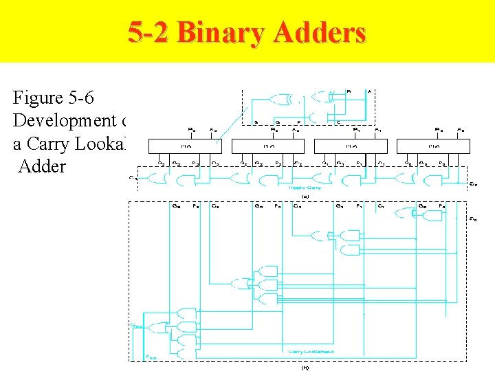
5 -2 Binary Adders Figure 5 -6 Development of a Carry Lookahead Adder

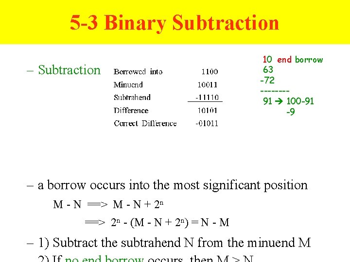
5 -3 Binary Subtraction – Subtraction 10 end borrow 63 -72 -------91 100 -91 -9 – a borrow occurs into the most significant position M - N ==> M - N + 2 n ==> 2 n - (M - N + 2 n) = N - M – 1) Subtract the subtrahend N from the minuend M

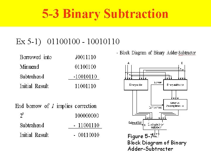
5 -3 Binary Subtraction Ex 5 -1) 01100100 - 10010110 Figure 5 -7 Block Diagram of Binary Adder-Subtracter

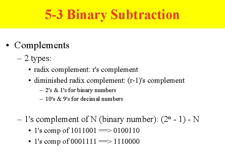
5 -3 Binary Subtraction • Complements – 2 types: • radix complement: r's complement • diminished radix complement: (r-1)'s complement – 2's & 1's for binary numbers – 10's & 9's for decimal numbers – 1's complement of N (binary number): (2 n - 1) - N • 1's comp of 1011001 ==> 0100110 • 1's comp of 0001111 ==> 1110000

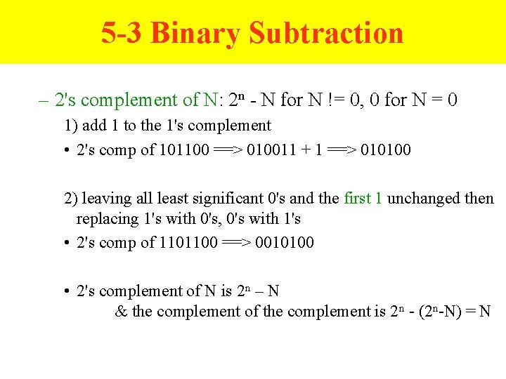
5 -3 Binary Subtraction – 2's complement of N: 2 n - N for N != 0, 0 for N = 0 1) add 1 to the 1's complement • 2's comp of 101100 ==> 010011 + 1 ==> 010100 2) leaving all least significant 0's and the first 1 unchanged then replacing 1's with 0's, 0's with 1's • 2's comp of 1101100 ==> 0010100 • 2's complement of N is 2 n – N & the complement of the complement is 2 n - (2 n-N) = N

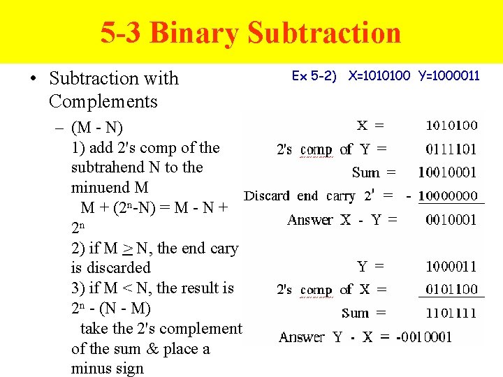
5 -3 Binary Subtraction • Subtraction with Complements – (M - N) 1) add 2's comp of the subtrahend N to the minuend M M + (2 n-N) = M - N + 2 n 2) if M > N, the end cary is discarded 3) if M < N, the result is 2 n - (N - M) take the 2's complement of the sum & place a minus sign Ex 5 -2) X=1010100 Y=1000011

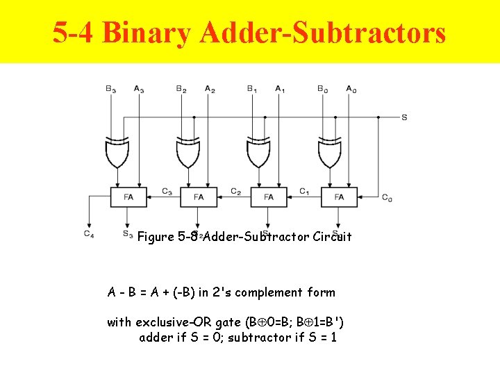
5 -4 Binary Adder-Subtractors Figure 5 -8 Adder-Subtractor Circuit A - B = A + (-B) in 2's complement form with exclusive-OR gate (B 0=B; B 1=B') adder if S = 0; subtractor if S = 1

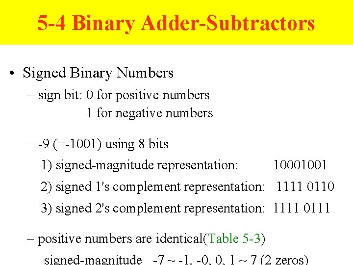
5 -4 Binary Adder-Subtractors • Signed Binary Numbers – sign bit: 0 for positive numbers 1 for negative numbers – -9 (=-1001) using 8 bits 1) signed-magnitude representation: 10001001 2) signed 1's complement representation: 1111 0110 3) signed 2's complement representation: 1111 0111 – positive numbers are identical(Table 5 -3) signed-magnitude -7 ~ -1, -0, 0, 1 ~ 7 (2 zeros)

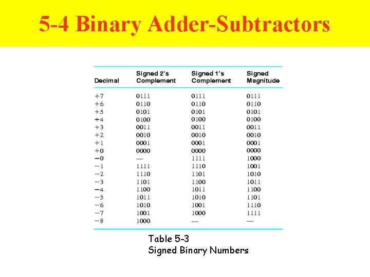
5 -4 Binary Adder-Subtractors Table 5 -3 Signed Binary Numbers

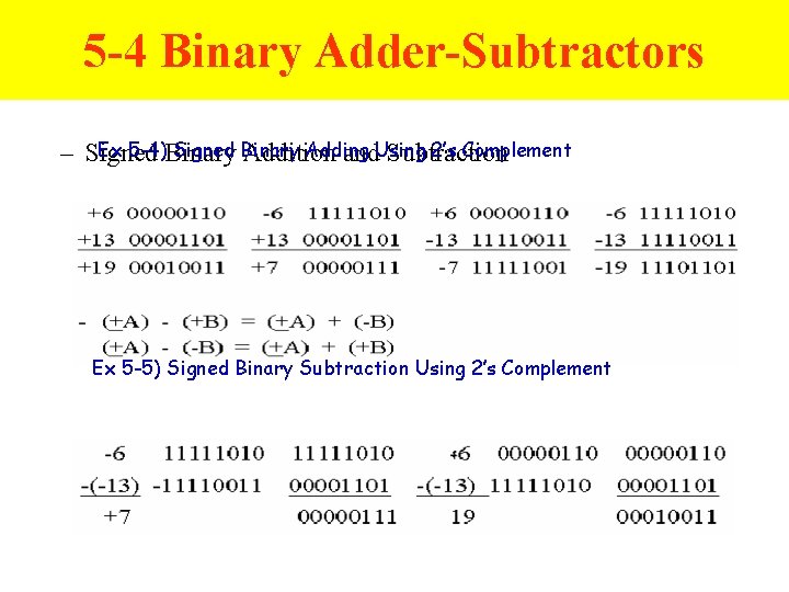
5 -4 Binary Adder-Subtractors Ex 5 -4)Binary Signed Binary Adding 2’s Complement – Signed Addition and. Using Subtraction Ex 5 -5) Signed Binary Subtraction Using 2’s Complement

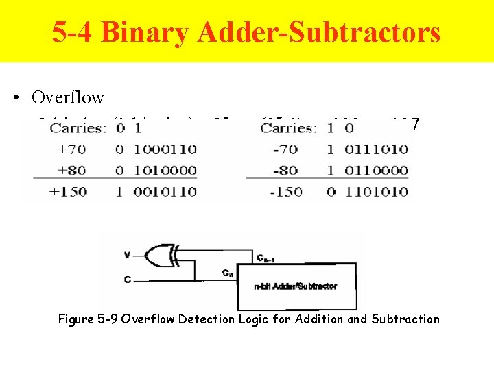
5 -4 Binary Adder-Subtractors • Overflow 8 -bit data(1 -bit sign): -27 ~ +(27 -1) = -128 ~ +127 Figure 5 -9 Overflow Detection Logic for Addition and Subtraction

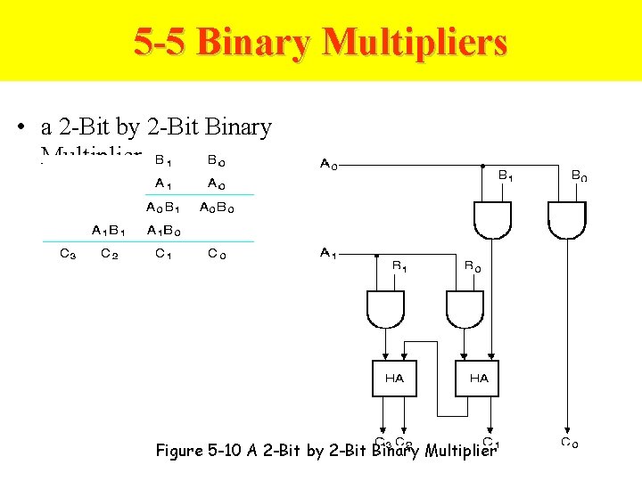
5 -5 Binary Multipliers • a 2 -Bit by 2 -Bit Binary Multiplier Figure 5 -10 A 2 -Bit by 2 -Bit Binary Multiplier

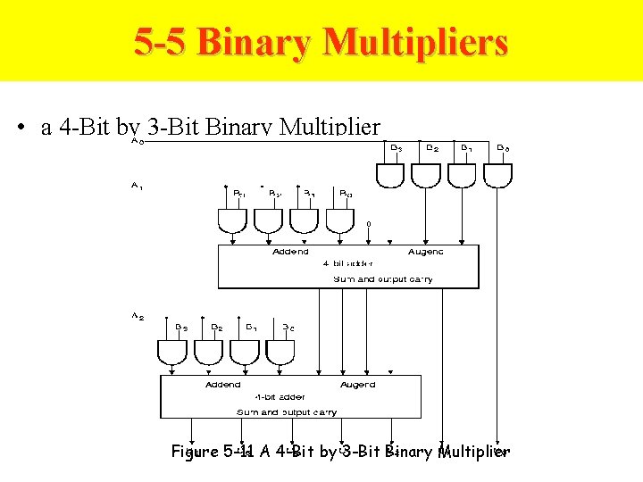
5 -5 Binary Multipliers • a 4 -Bit by 3 -Bit Binary Multiplier Figure 5 -11 A 4 -Bit by 3 -Bit Binary Multiplier

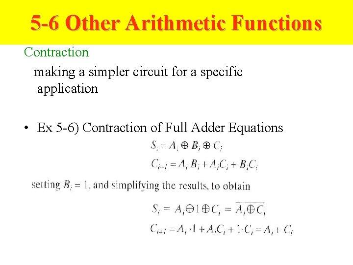
5 -6 Other Arithmetic Functions Contraction making a simpler circuit for a specific application • Ex 5 -6) Contraction of Full Adder Equations

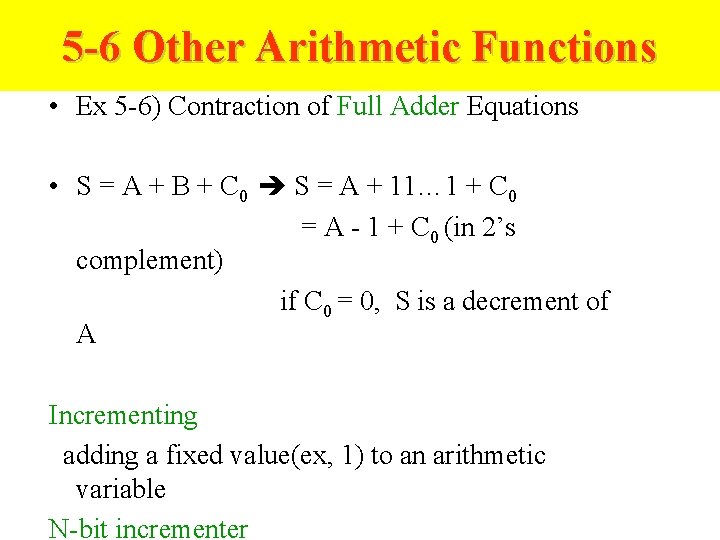
5 -6 Other Arithmetic Functions • Ex 5 -6) Contraction of Full Adder Equations • S = A + B + C 0 S = A + 11… 1 + C 0 = A - 1 + C 0 (in 2’s complement) if C 0 = 0, S is a decrement of A Incrementing adding a fixed value(ex, 1) to an arithmetic variable N-bit incrementer

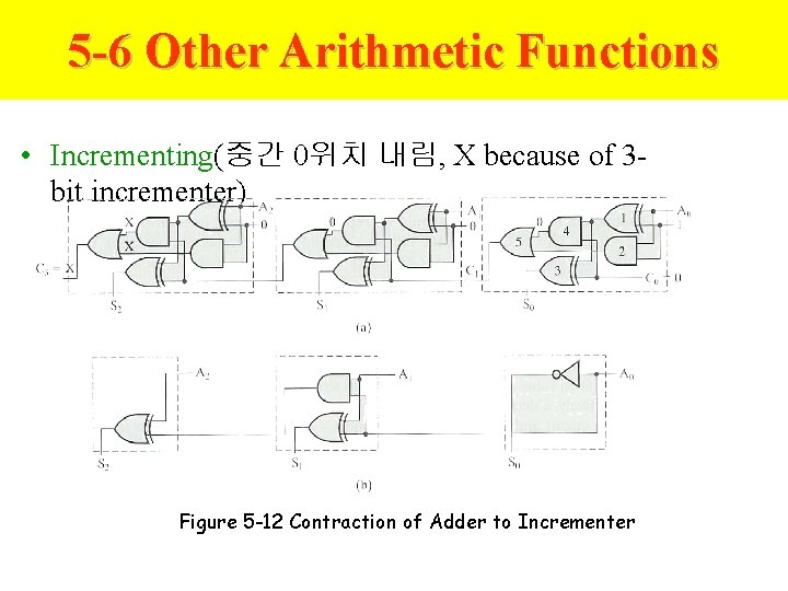
5 -6 Other Arithmetic Functions • Incrementing(중간 0위치 내림, X because of 3 bit incrementer) Figure 5 -12 Contraction of Adder to Incrementer

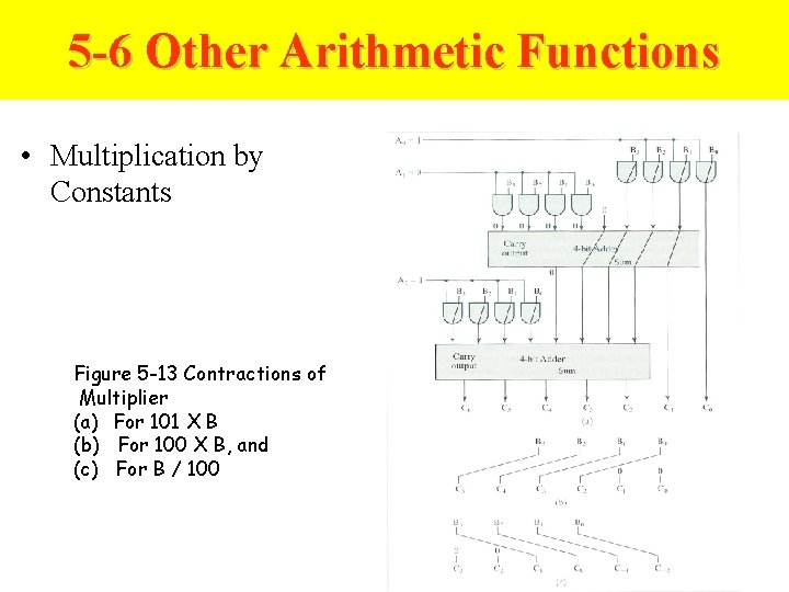
5 -6 Other Arithmetic Functions • Multiplication by Constants Figure 5 -13 Contractions of Multiplier (a) For 101 X B (b) For 100 X B, and (c) For B / 100

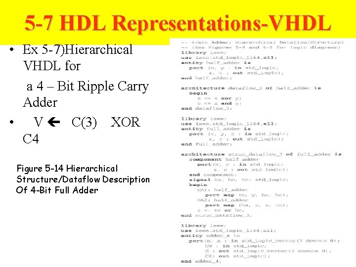
5 -7 HDL Representations-VHDL • Ex 5 -7)Hierarchical VHDL for a 4 – Bit Ripple Carry Adder • V C(3) XOR C 4 Figure 5 -14 Hierarchical Structure/Dataflow Description Of 4 -Bit Full Adder

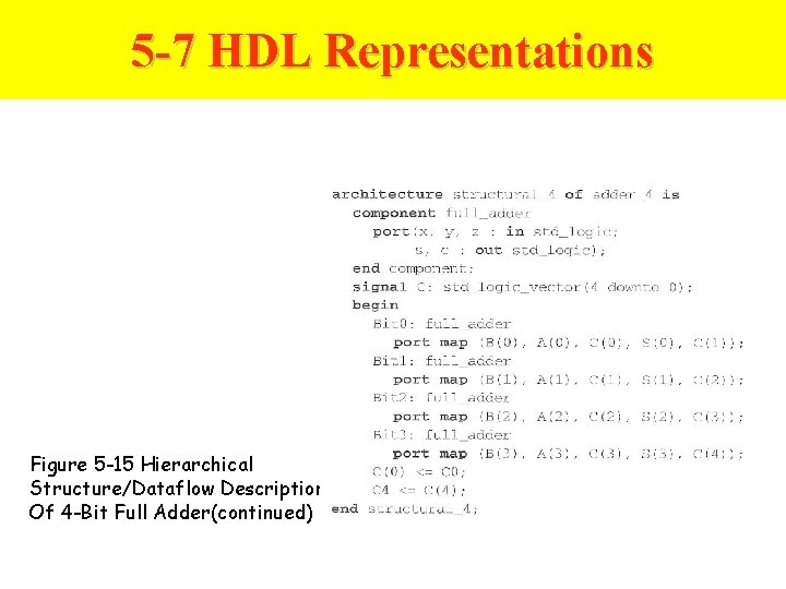
5 -7 HDL Representations Figure 5 -15 Hierarchical Structure/Dataflow Description Of 4 -Bit Full Adder(continued)

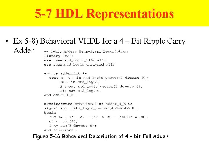
5 -7 HDL Representations • Ex 5 -8) Behavioral VHDL for a 4 – Bit Ripple Carry Adder Figure 5 -16 Behavioral Description of 4 – bit Full Adder

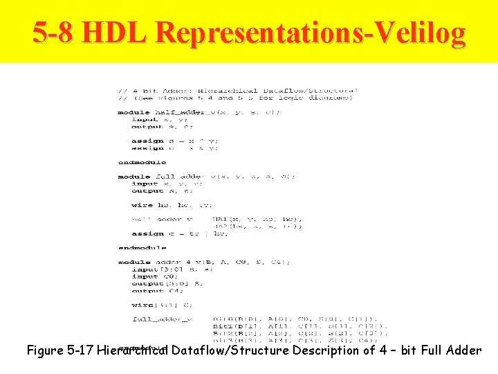
5 -8 HDL Representations-Velilog Figure 5 -17 Hierarchical Dataflow/Structure Description of 4 – bit Full Adder

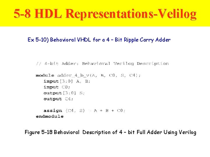
5 -8 HDL Representations-Velilog Ex 5 -10) Behavioral VHDL for a 4 – Bit Ripple Carry Adder Figure 5 -18 Behavioral Description of 4 – bit Full Adder Using Verilog