Introduction CS 46101 Section 600 CS 56101 Section

Introduction CS 46101 Section 600 CS 56101 Section 002 Dr. Angela Guercio Spring 2010

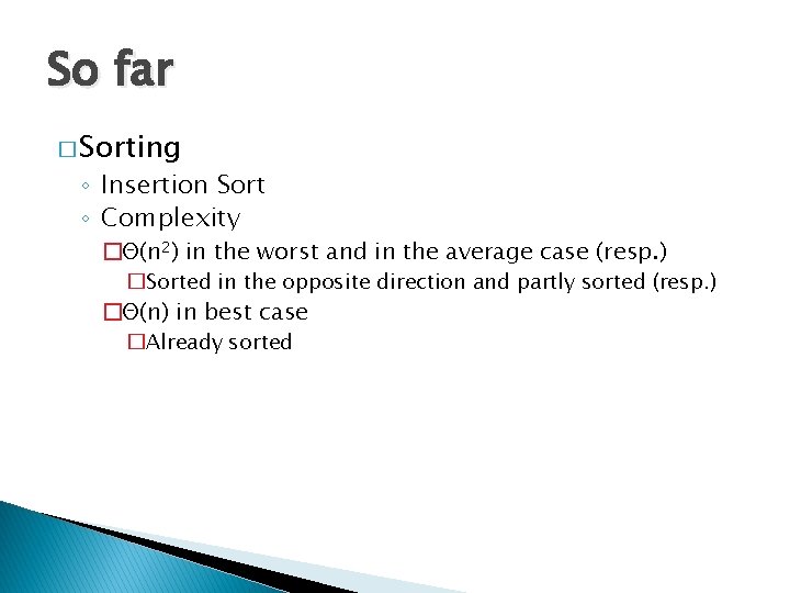
So far � Sorting ◦ Insertion Sort ◦ Complexity �Θ(n 2) in the worst and in the average case (resp. ) �Sorted in the opposite direction and partly sorted (resp. ) �Θ(n) in best case �Already sorted

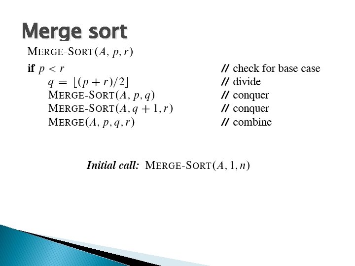
Merge sort � To sort A[p. . r]: ◦ Divide by splitting into two subarrays A[p. . q] and A[q + 1. . r], where q is the halfway point of A[p. . r]. ◦ Conquer by recursively sorting the two subarrays A[p. . q] and A[q + 1. . r]. ◦ Combine by merging the two sorted subarrays A[p. . q] and A[q + 1. . r] to produce a single sorted subarray A[p. . r]. To accomplish this step, we’ll define a procedure MERGE(A, p, q, r). ◦ The recursion bottoms out when the subarray has just 1 element, so that it’s trivially sorted.

Merge sort

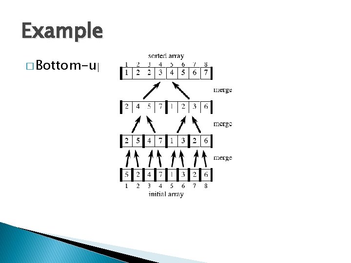
Example � Bottom-up view for n = 8

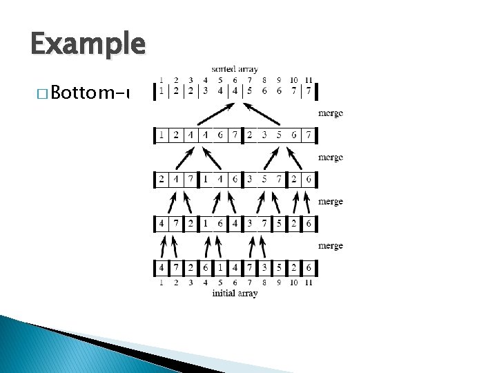
Example � Bottom-up view for n = 11

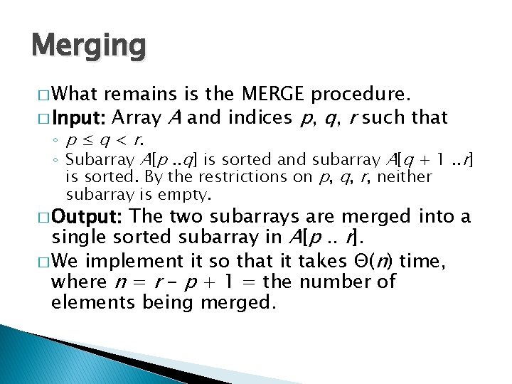
Merging � What remains is the MERGE procedure. � Input: Array A and indices p, q, r such that ◦ p ≤ q < r. ◦ Subarray A[p. . q] is sorted and subarray A[q + 1. . r] is sorted. By the restrictions on p, q, r, neither subarray is empty. � Output: The two subarrays are merged into a single sorted subarray in A[p. . r]. � We implement it so that it takes Θ(n) time, where n = r - p + 1 = the number of elements being merged.

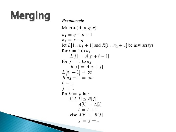
Merging

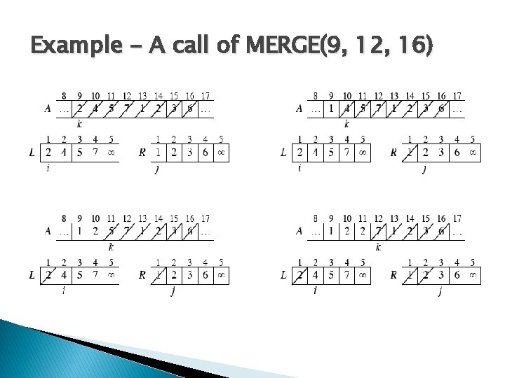
Example - A call of MERGE(9, 12, 16)

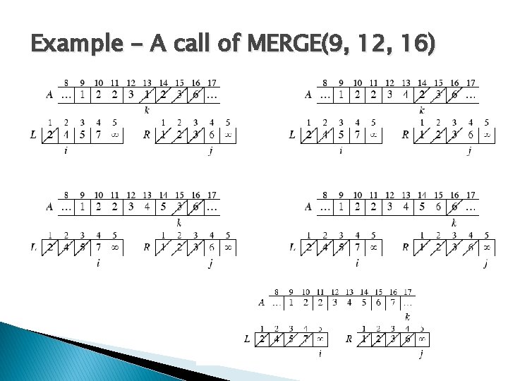
Example - A call of MERGE(9, 12, 16)

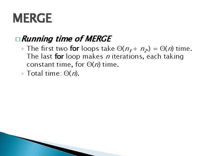
MERGE � Running time of MERGE ◦ The first two for loops take Θ(n 1 + n 2 ) = Θ(n) time. The last for loop makes n iterations, each taking constant time, for Θ(n) time. ◦ Total time: Θ(n). 1 22

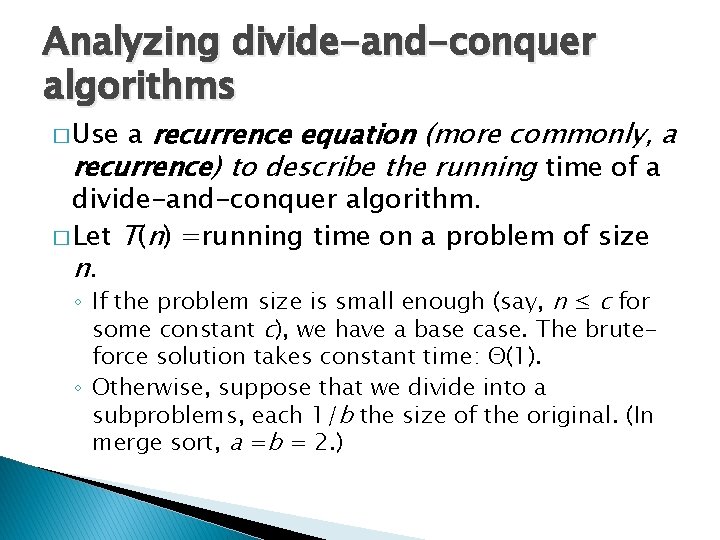
Analyzing divide-and-conquer algorithms a recurrence equation (more commonly, a recurrence) to describe the running time of a divide-and-conquer algorithm. � Let T(n) =running time on a problem of size n. � Use ◦ If the problem size is small enough (say, n ≤ c for some constant c), we have a base case. The bruteforce solution takes constant time: Θ(1). ◦ Otherwise, suppose that we divide into a subproblems, each 1/b the size of the original. (In merge sort, a =b = 2. )

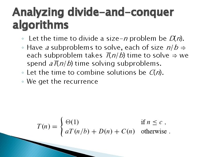
Analyzing divide-and-conquer algorithms ◦ Let the time to divide a size-n problem be D(n). ◦ Have a subproblems to solve, each of size n/b ⇒ each subproblem takes T(n/b) time to solve ⇒ we spend a. T(n/b) time solving subproblems. ◦ Let the time to combine solutions be C(n). ◦ We get the recurrence

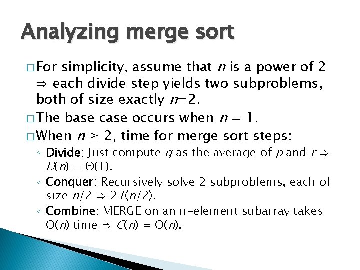
Analyzing merge sort simplicity, assume that n is a power of 2 ⇒ each divide step yields two subproblems, both of size exactly n=2. � The base case occurs when n = 1. � When n ≥ 2, time for merge sort steps: � For ◦ Divide: Just compute q as the average of p and r ⇒ D(n) = Θ(1). ◦ Conquer: Recursively solve 2 subproblems, each of size n/2 ⇒ 2 T(n/2). ◦ Combine: MERGE on an n-element subarray takes Θ(n) time ⇒ C(n) = Θ(n).

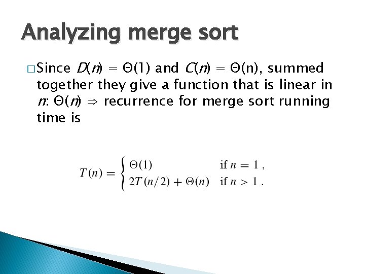
Analyzing merge sort � Since D(n) = Θ(1) and C(n) = Θ(n), summed together they give a function that is linear in n: Θ(n) ⇒ recurrence for merge sort running time is

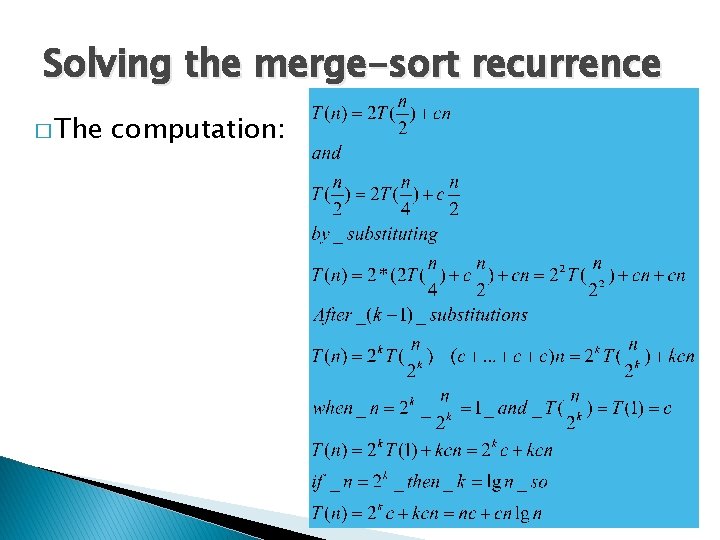
Solving the merge-sort recurrence � By the master theorem in Chapter 4, we can show that this recurrence has the solution T(n) =Θ(n lg n). � Compared to insertion sort Θ(n 2) worst-case time), merge sort is faster. � On small inputs, insertion sort may be faster. � We can understand how to solve the mergesort recurrence without the master theorem.

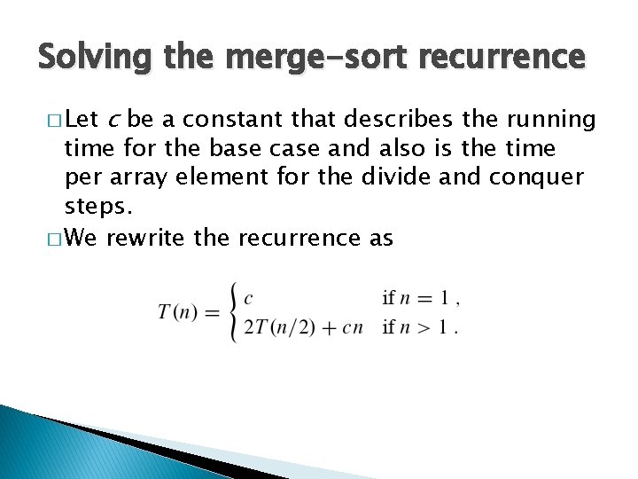
Solving the merge-sort recurrence � Let c be a constant that describes the running time for the base case and also is the time per array element for the divide and conquer steps. � We rewrite the recurrence as

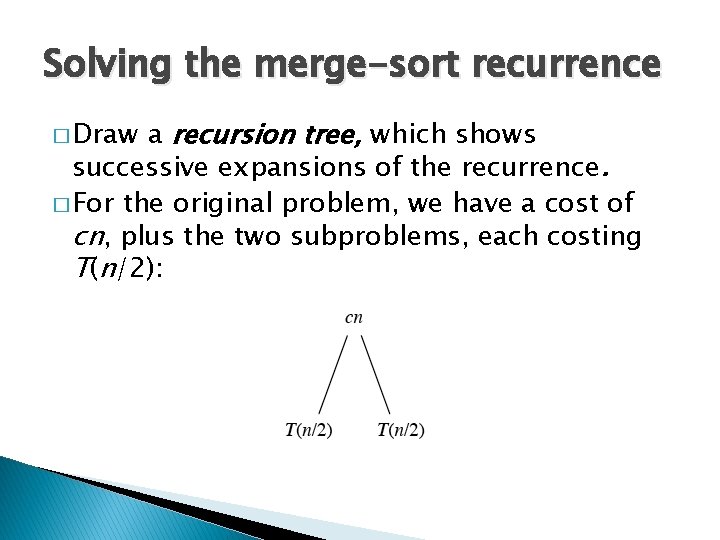
Solving the merge-sort recurrence a recursion tree, which shows successive expansions of the recurrence. � For the original problem, we have a cost of cn, plus the two subproblems, each costing T(n/2): � Draw

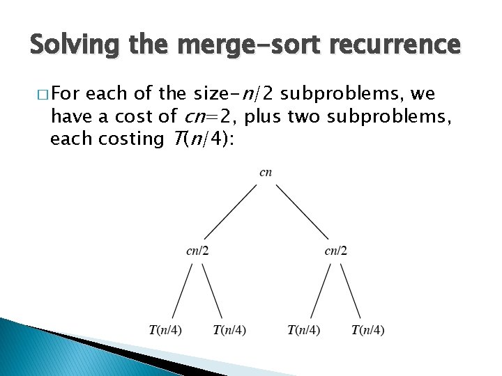
Solving the merge-sort recurrence each of the size-n/2 subproblems, we have a cost of cn=2, plus two subproblems, each costing T(n/4): � For

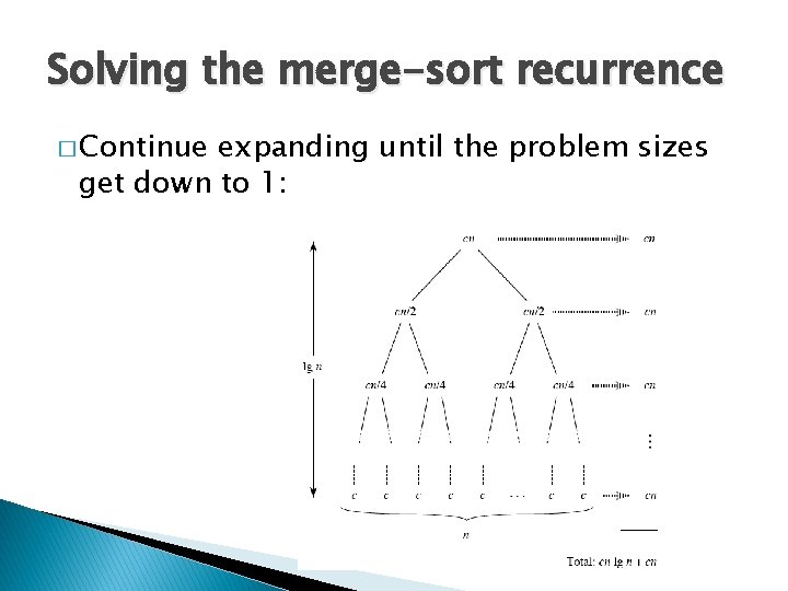
Solving the merge-sort recurrence � Continue expanding until the problem sizes get down to 1:

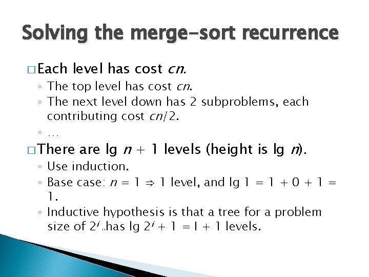
Solving the merge-sort recurrence � Each level has cost cn. ◦ The top level has cost cn. ◦ The next level down has 2 subproblems, each contributing cost cn/2. ◦ … � There are lg n + 1 levels (height is lg n). ◦ Use induction. ◦ Base case: n = 1 ⇒ 1 level, and lg 1 = 1 + 0 + 1 = 1. ◦ Inductive hypothesis is that a tree for a problem size of 2 i has lg 2 i + 1 = I + 1 levels. i I

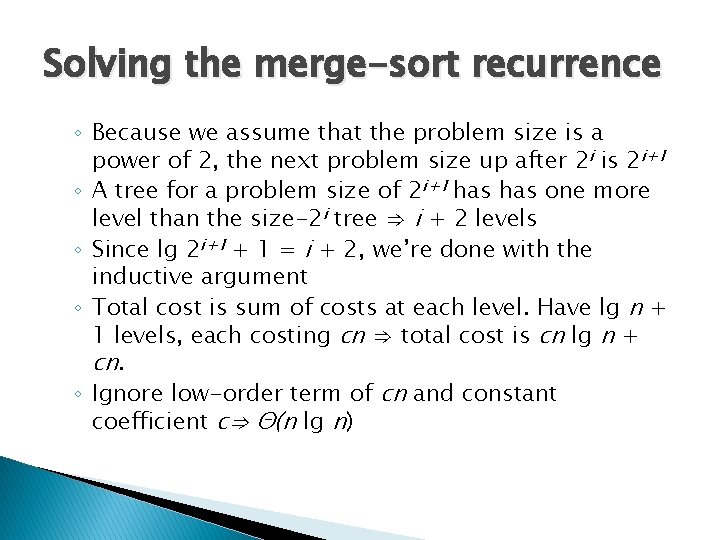
Solving the merge-sort recurrence ◦ Because we assume that the problem size is a power of 2, the next problem size up after 2 i is 2 i+1 ◦ A tree for a problem size of 2 i+1 has one more level than the size-2 i tree ⇒ i + 2 levels ◦ Since lg 2 i+1 + 1 = i + 2, we’re done with the inductive argument ◦ Total cost is sum of costs at each level. Have lg n + 1 levels, each costing cn ⇒ total cost is cn lg n + cn. ◦ Ignore low-order term of cn and constant coefficient c⇒ Θ(n lg n)

Solving the merge-sort recurrence � The computation:

Next Time � Growth of functions � Reading: ◦ Read Chapter 3