Introduction Applications Optimality Conditions Primal Dual in LP











- Slides: 79

Introduction Applications Optimality Conditions Primal Dual in LP Algorithms Ben Klein – 11/03/13 MINIMUM COST FLOWS: INTRODUCTION AND BASIC ALGORITHMS

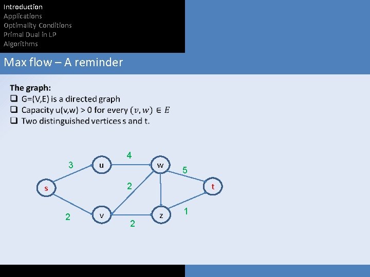
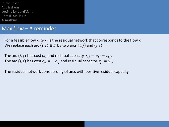
Introduction Applications Optimality Conditions Primal Dual in LP Algorithms Max flow – A reminder 3 u 4 w 5 t 2 s 2 v 2 z 1

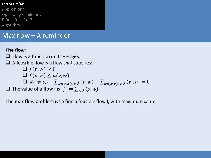
Introduction Applications Optimality Conditions Primal Dual in LP Algorithms Max flow – A reminder

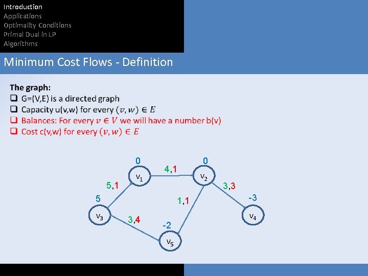
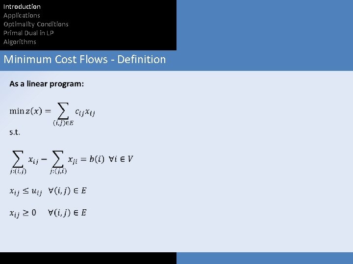
Introduction Applications Optimality Conditions Primal Dual in LP Algorithms Minimum Cost Flows - Definition 0 5, 1 v 1 4, 1 5 v 3 1, 1 3, 4 -2 v 5 0 v 2 3, 3 -3 v 4

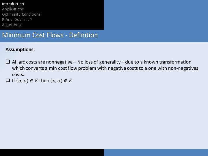
Introduction Applications Optimality Conditions Primal Dual in LP Algorithms Minimum Cost Flows - Definition

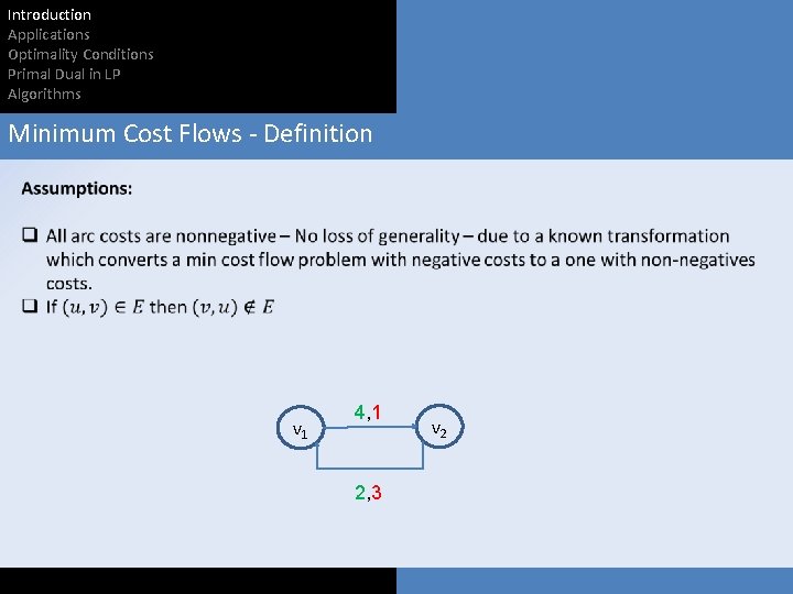
Introduction Applications Optimality Conditions Primal Dual in LP Algorithms Minimum Cost Flows - Definition v 1 4, 1 2, 3 v 2

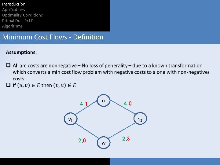
Introduction Applications Optimality Conditions Primal Dual in LP Algorithms Minimum Cost Flows - Definition 4, 1 u 4, 0 v 2 v 1 2, 0 w 2, 3

Introduction Applications Optimality Conditions Primal Dual in LP Algorithms Minimum Cost Flows - Definition

Introduction Applications Optimality Conditions Primal Dual in LP Algorithms Max flow – A reminder

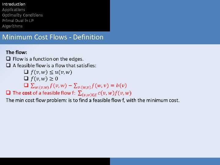
Introduction Applications Optimality Conditions Primal Dual in LP Algorithms Minimum Cost Flows - Definition

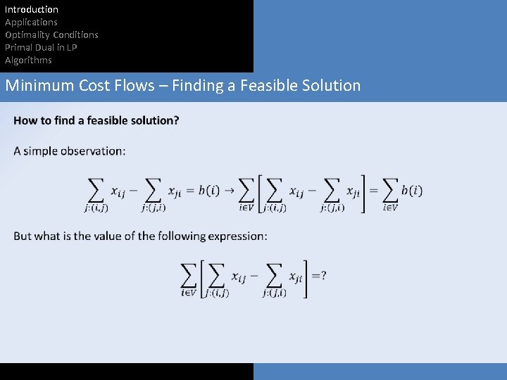
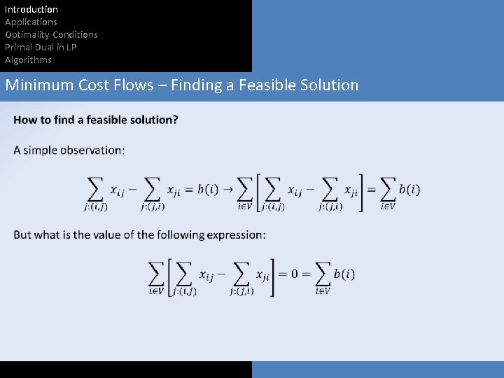
Introduction Applications Optimality Conditions Primal Dual in LP Algorithms Minimum Cost Flows – Finding a Feasible Solution

Introduction Applications Optimality Conditions Primal Dual in LP Algorithms Minimum Cost Flows – Finding a Feasible Solution

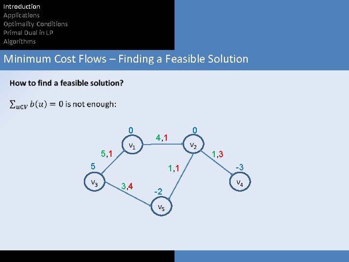
Introduction Applications Optimality Conditions Primal Dual in LP Algorithms Minimum Cost Flows – Finding a Feasible Solution 0 5, 1 v 1 4, 1 5 v 3 1, 1 3, 4 -2 v 5 0 v 2 1, 3 -3 v 4

Introduction Applications Optimality Conditions Primal Dual in LP Algorithms Minimum Cost Flows – Finding a Feasible Solution 0 5, 1 v 1 4, 1 5 v 3 1, 1 3, 4 -2 v 5 0 v 2 3, 3 -3 v 4

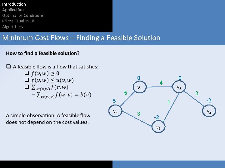
Introduction Applications Optimality Conditions Primal Dual in LP Algorithms Minimum Cost Flows – Finding a Feasible Solution 0 5 4 v 1 5 v 3 0 v 2 1 3 -2 v 5 3 -3 v 4

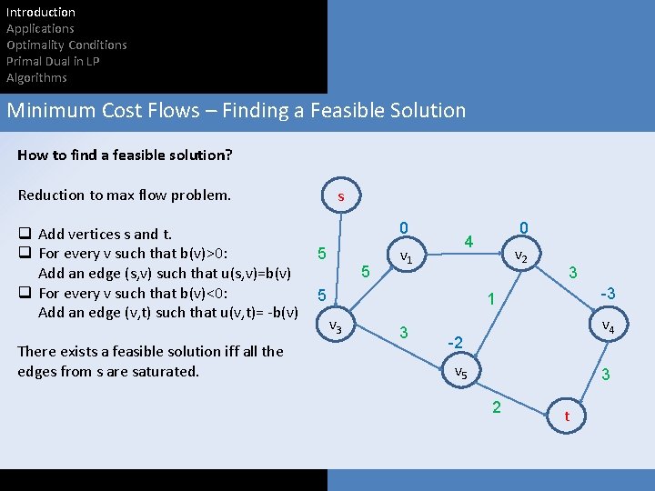
Introduction Applications Optimality Conditions Primal Dual in LP Algorithms Minimum Cost Flows – Finding a Feasible Solution How to find a feasible solution? Reduction to max flow problem. q Add vertices s and t. q For every v such that b(v)>0: Add an edge (s, v) such that u(s, v)=b(v) q For every v such that b(v)<0: Add an edge (v, t) such that u(v, t)= -b(v) There exists a feasible solution iff all the edges from s are saturated. s 0 5 5 0 4 v 1 5 v 2 3 -3 1 v 3 3 v 4 -2 v 5 3 2 t

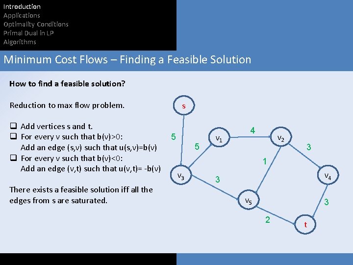
Introduction Applications Optimality Conditions Primal Dual in LP Algorithms Minimum Cost Flows – Finding a Feasible Solution How to find a feasible solution? Reduction to max flow problem. q Add vertices s and t. q For every v such that b(v)>0: Add an edge (s, v) such that u(s, v)=b(v) q For every v such that b(v)<0: Add an edge (v, t) such that u(v, t)= -b(v) There exists a feasible solution iff all the edges from s are saturated. s 5 5 v 1 4 v 2 3 1 v 3 v 4 3 v 5 3 2 t

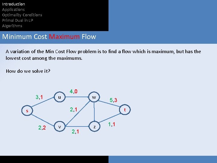
Introduction Applications Optimality Conditions Primal Dual in LP Algorithms Minimum Cost Maximum Flow A variation of the Min Cost Flow problem is to find a flow which is maximum, but has the lowest cost among the maximums. How do we solve it? 3, 1 u 4, 0 w 5, 3 t 2, 1 s 2, 2 v 2, 1 z 1, 1

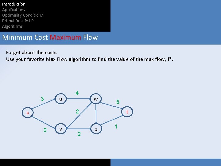
Introduction Applications Optimality Conditions Primal Dual in LP Algorithms Minimum Cost Maximum Flow Forget about the costs. Use your favorite Max Flow algorithm to find the value of the max flow, f*. 3 u 4 w 5 t 2 s 2 v 2 z 1

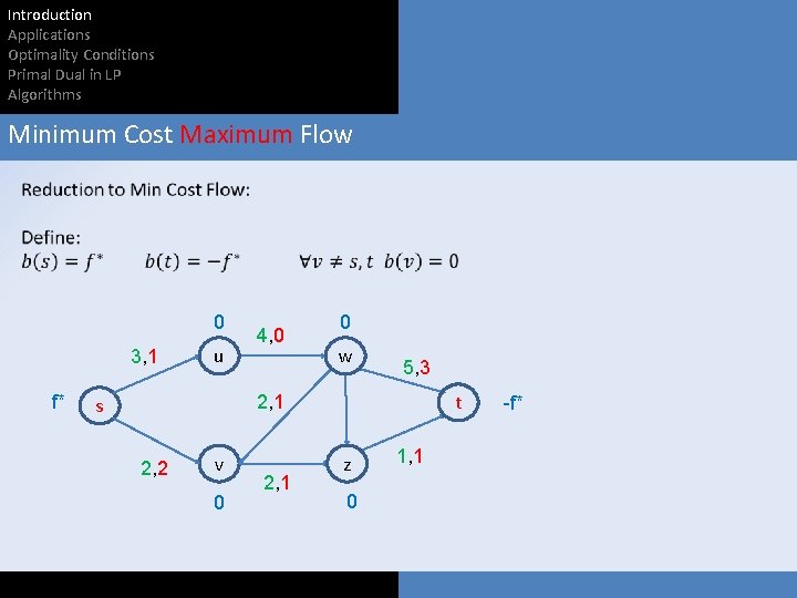
Introduction Applications Optimality Conditions Primal Dual in LP Algorithms Minimum Cost Maximum Flow 0 3, 1 f* u 4, 0 0 w 5, 3 t 2, 1 s 2, 2 v 0 2, 1 z 0 1, 1 -f*

Introduction Applications Optimality Conditions Primal Dual in LP Algorithms Minimum Cost Flow – Application #1

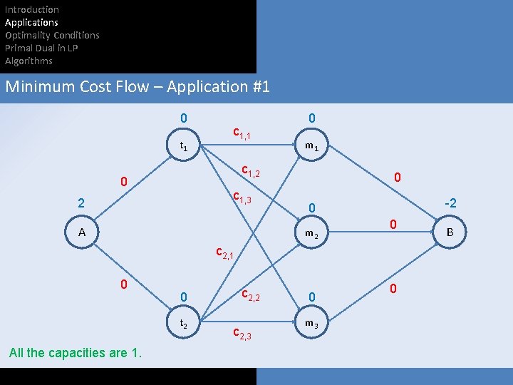
Introduction Applications Optimality Conditions Primal Dual in LP Algorithms Minimum Cost Flow – Application #1 0 t 1 c 1, 1 0 m 1 c 1, 2 0 c 1, 3 2 A 0 -2 0 m 2 0 c 2, 1 0 0 t 2 All the capacities are 1. c 2, 2 c 2, 3 0 m 3 0 B

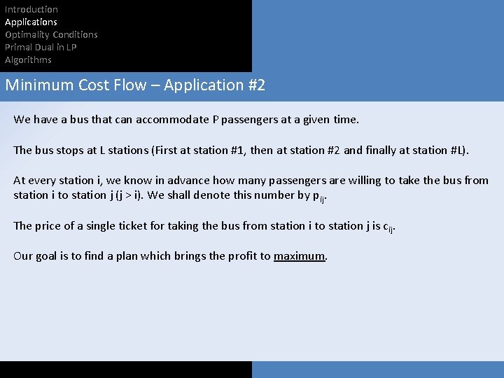
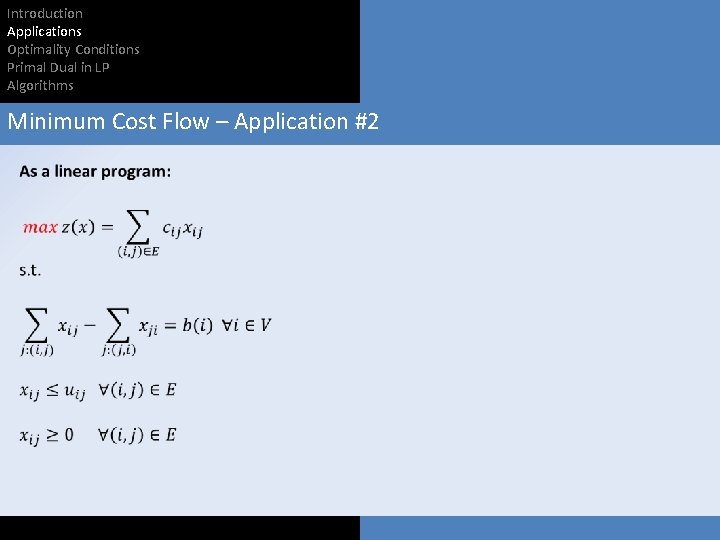
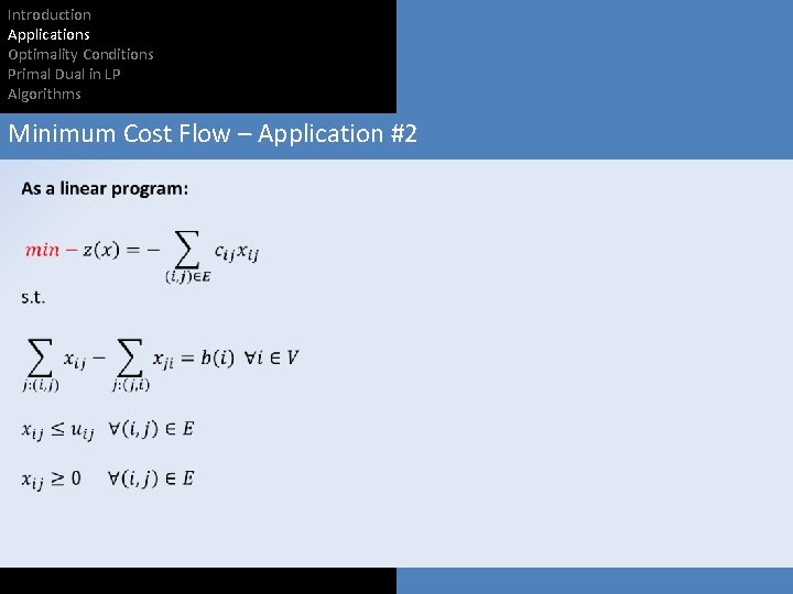
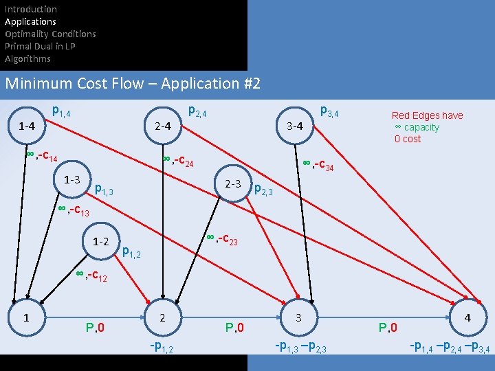
Introduction Applications Optimality Conditions Primal Dual in LP Algorithms Minimum Cost Flow – Application #2 We have a bus that can accommodate P passengers at a given time. The bus stops at L stations (First at station #1, then at station #2 and finally at station #L). At every station i, we know in advance how many passengers are willing to take the bus from station i to station j (j > i). We shall denote this number by pij. The price of a single ticket for taking the bus from station i to station j is c ij. Our goal is to find a plan which brings the profit to maximum.

Introduction Applications Optimality Conditions Primal Dual in LP Algorithms Minimum Cost Flow – Application #2

Introduction Applications Optimality Conditions Primal Dual in LP Algorithms Minimum Cost Flow – Application #2

Introduction Applications Optimality Conditions Primal Dual in LP Algorithms Minimum Cost Flow – Application #2

Introduction Applications Optimality Conditions Primal Dual in LP Algorithms Minimum Cost Flow – Application #2

Introduction Applications Optimality Conditions Primal Dual in LP Algorithms Minimum Cost Flow – Application #2 1 -4 p 1, 4 2 -4 ∞, -c 14 p 2, 4 3 -4 ∞, -c 24 1 -3 p 3, 4 Red Edges have ∞ capacity 0 cost ∞, -c 34 p 1, 3 2 -3 1 -2 ∞, -c 23 p 2, 3 ∞, -c 13 p 1, 2 ∞, -c 12 1 P, 0 2 -p 1, 2 P, 0 3 -p 1, 3 –p 2, 3 P, 0 4 -p 1, 4 –p 2, 4 –p 3, 4

Introduction Applications Optimality Conditions Primal Dual in LP Algorithms Minimum Cost Flow – Optimality Conditions We’ll consider three different optimality conditions: q Negative cycle q Reduced cost q Complementary slackness

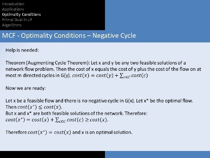
Introduction Applications Optimality Conditions Primal Dual in LP Algorithms MCF - Optimality Conditions – Negative Cycle Theorem: A feasible solution x* is an optimal solution of the MCF problem if and only if it satisfies the negative cycle optimality conditions: namely, the residual network G(x*) contains no negative cost (directed) cycle.

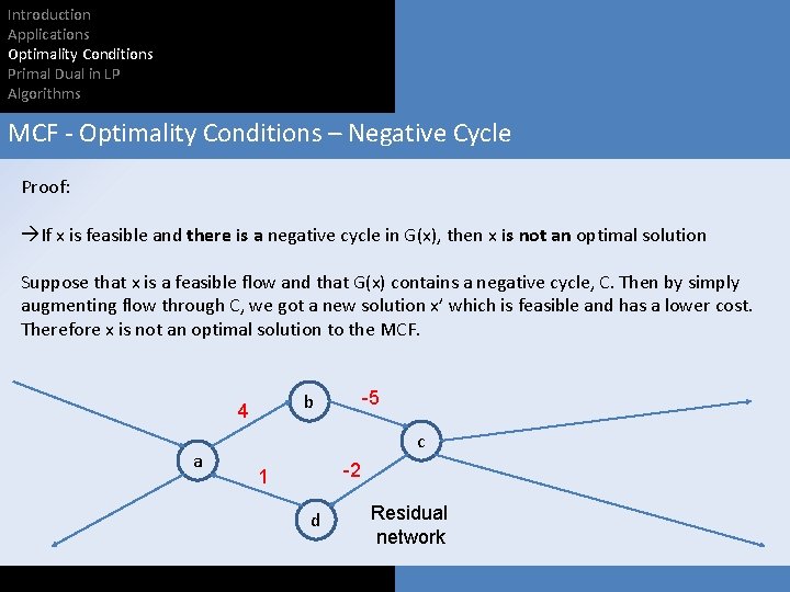
Introduction Applications Optimality Conditions Primal Dual in LP Algorithms MCF - Optimality Conditions – Negative Cycle Proof: If x is feasible and there is a negative cycle in G(x), then x is not an optimal solution Suppose that x is a feasible flow and that G(x) contains a negative cycle, C. Then by simply augmenting flow through C, we got a new solution x’ which is feasible and has a lower cost. Therefore x is not an optimal solution to the MCF. a -5 b 4 c -2 1 d Residual network

Introduction Applications Optimality Conditions Primal Dual in LP Algorithms MCF - Optimality Conditions – Negative Cycle Proof: If x is feasible and there is no negative cycle in G(x), then x is an optimal solution

Introduction Applications Optimality Conditions Primal Dual in LP Algorithms MCF - Optimality Conditions – Negative Cycle

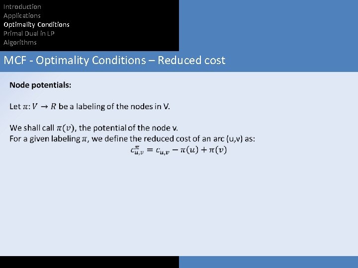
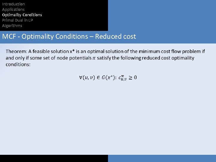
Introduction Applications Optimality Conditions Primal Dual in LP Algorithms MCF - Optimality Conditions – Reduced cost

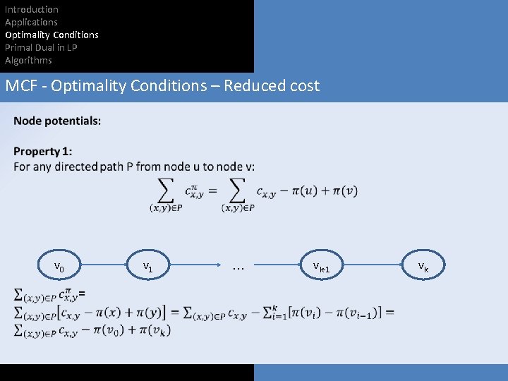
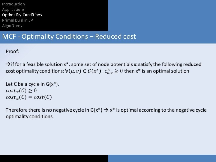
Introduction Applications Optimality Conditions Primal Dual in LP Algorithms MCF - Optimality Conditions – Reduced cost v 0 v 1 … vk-1 vk

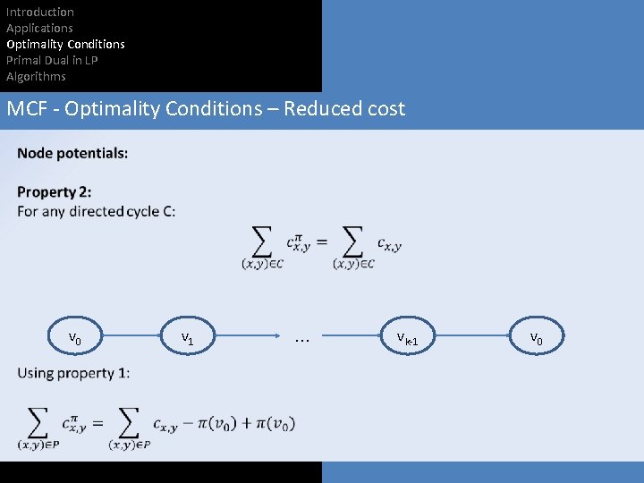
Introduction Applications Optimality Conditions Primal Dual in LP Algorithms MCF - Optimality Conditions – Reduced cost v 0 v 1 … vk-1 v 0

Introduction Applications Optimality Conditions Primal Dual in LP Algorithms MCF - Optimality Conditions – Reduced cost

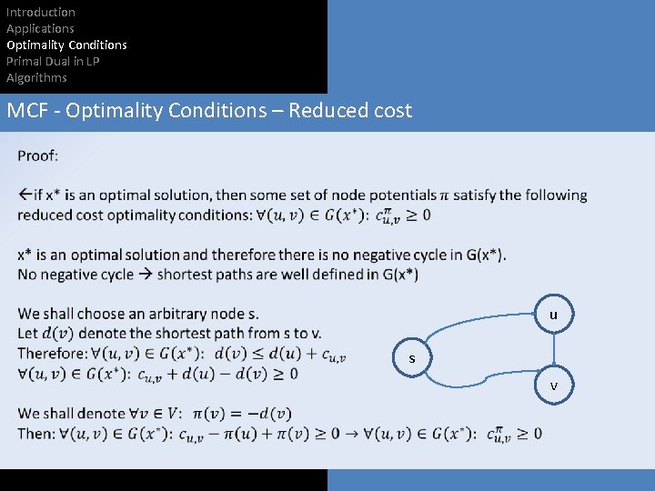
Introduction Applications Optimality Conditions Primal Dual in LP Algorithms MCF - Optimality Conditions – Reduced cost

Introduction Applications Optimality Conditions Primal Dual in LP Algorithms MCF - Optimality Conditions – Reduced cost u s v

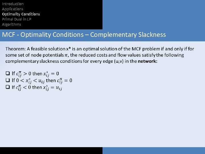
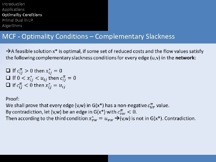
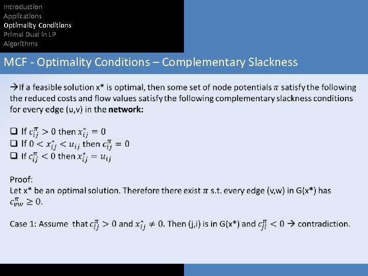
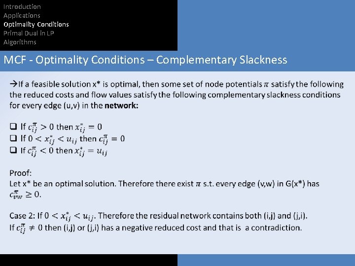
Introduction Applications Optimality Conditions Primal Dual in LP Algorithms MCF - Optimality Conditions – Complementary Slackness

Introduction Applications Optimality Conditions Primal Dual in LP Algorithms MCF - Optimality Conditions – Complementary Slackness

Introduction Applications Optimality Conditions Primal Dual in LP Algorithms MCF - Optimality Conditions – Complementary Slackness

Introduction Applications Optimality Conditions Primal Dual in LP Algorithms MCF - Optimality Conditions – Complementary Slackness

Introduction Applications Optimality Conditions Primal Dual in LP Algorithms MCF - Optimality Conditions – Complementary Slackness

Introduction Applications Optimality Conditions Primal Dual in LP Algorithms PRIMAL DUAL IN LP

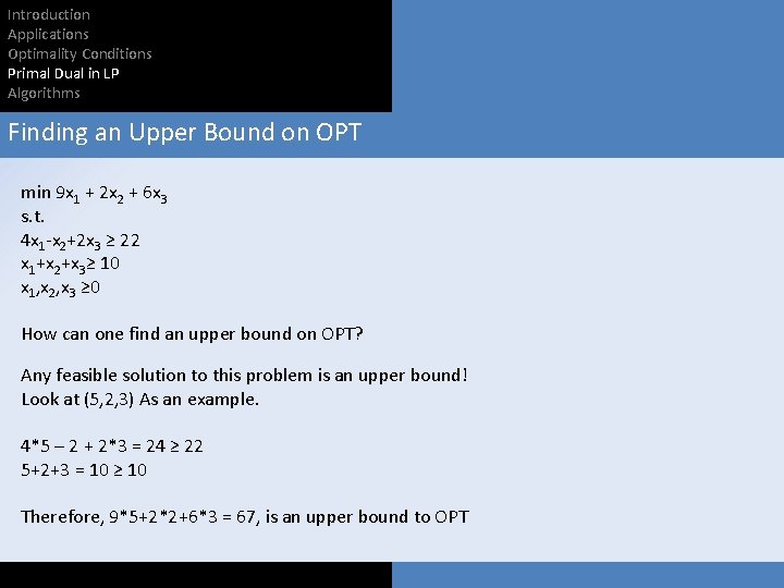
Introduction Applications Optimality Conditions Primal Dual in LP Algorithms Finding an Upper Bound on OPT min 9 x 1 + 2 x 2 + 6 x 3 s. t. 4 x 1 -x 2+2 x 3 ≥ 22 x 1+x 2+x 3≥ 10 x 1, x 2, x 3 ≥ 0 How can one find an upper bound on OPT? Any feasible solution to this problem is an upper bound! Look at (5, 2, 3) As an example. 4*5 – 2 + 2*3 = 24 ≥ 22 5+2+3 = 10 ≥ 10 Therefore, 9*5+2*2+6*3 = 67, is an upper bound to OPT

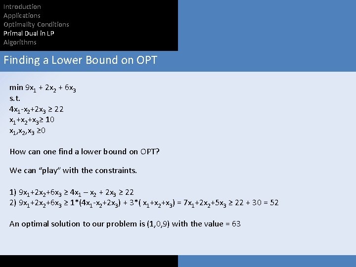
Introduction Applications Optimality Conditions Primal Dual in LP Algorithms Finding a Lower Bound on OPT min 9 x 1 + 2 x 2 + 6 x 3 s. t. 4 x 1 -x 2+2 x 3 ≥ 22 x 1+x 2+x 3≥ 10 x 1, x 2, x 3 ≥ 0 How can one find a lower bound on OPT? We can “play” with the constraints. 1) 9 x 1+2 x 2+6 x 3 ≥ 4 x 1 – x 2 + 2 x 3 ≥ 22 2) 9 x 1+2 x 2+6 x 3 ≥ 1*(4 x 1 -x 2+2 x 3) + 3*( x 1+x 2+x 3) = 7 x 1+2 x 2+5 x 3 ≥ 22 + 30 = 52 An optimal solution to our problem is (1, 0, 9) with the value = 63

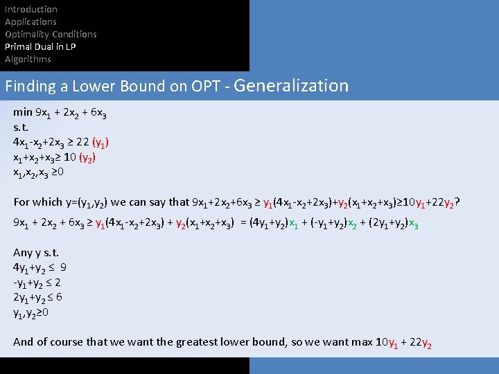
Introduction Applications Optimality Conditions Primal Dual in LP Algorithms Finding a Lower Bound on OPT - Generalization min 9 x 1 + 2 x 2 + 6 x 3 s. t. 4 x 1 -x 2+2 x 3 ≥ 22 (y 1) x 1+x 2+x 3≥ 10 (y 2) x 1, x 2, x 3 ≥ 0 For which y=(y 1, y 2) we can say that 9 x 1+2 x 2+6 x 3 ≥ y 1(4 x 1 -x 2+2 x 3)+y 2(x 1+x 2+x 3)≥ 10 y 1+22 y 2? 9 x 1 + 2 x 2 + 6 x 3 ≥ y 1(4 x 1 -x 2+2 x 3) + y 2(x 1+x 2+x 3) = (4 y 1+y 2)x 1 + (-y 1+y 2)x 2 + (2 y 1+y 2)x 3 Any y s. t. 4 y 1+y 2 ≤ 9 -y 1+y 2 ≤ 2 2 y 1+y 2 ≤ 6 y 1, y 2≥ 0 And of course that we want the greatest lower bound, so we want max 10 y 1 + 22 y 2

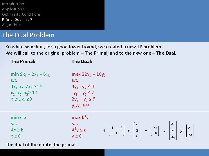
Introduction Applications Optimality Conditions Primal Dual in LP Algorithms The Dual Problem So while searching for a good lower bound, we created a new LP problem. We will call to the original problem – The Primal, and to the new one – The Dual. The Primal: The Dual: min 9 x 1 + 2 x 2 + 6 x 3 s. t. 4 x 1 -x 2+2 x 3 ≥ 22 x 1+x 2+x 3≥ 10 x 1, x 2, x 3 ≥ 0 max 22 y 1 + 10 y 2 s. t. 4 y 1 +y 2 ≤ 9 -y 1 + y 2 ≤ 2 2 y 1 + y 2 ≤ 6 y 1, y 2 ≥ 0 min c. Tx s. t. Ax ≥ b x≥ 0 max b. Ty s. t. ATy ≤ c y≥ 0 The dual of the dual is the primal

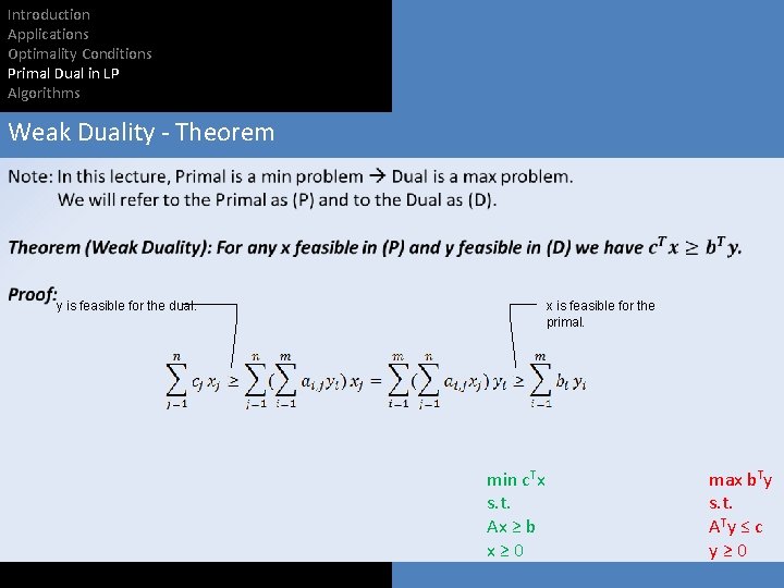
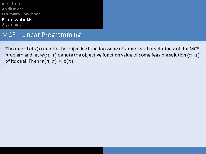
Introduction Applications Optimality Conditions Primal Dual in LP Algorithms Weak Duality - Theorem y is feasible for the dual. x is feasible for the primal. min c. Tx s. t. Ax ≥ b x≥ 0 max b. Ty s. t. ATy ≤ c y≥ 0

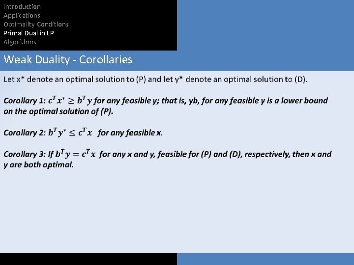
Introduction Applications Optimality Conditions Primal Dual in LP Algorithms Weak Duality - Corollaries

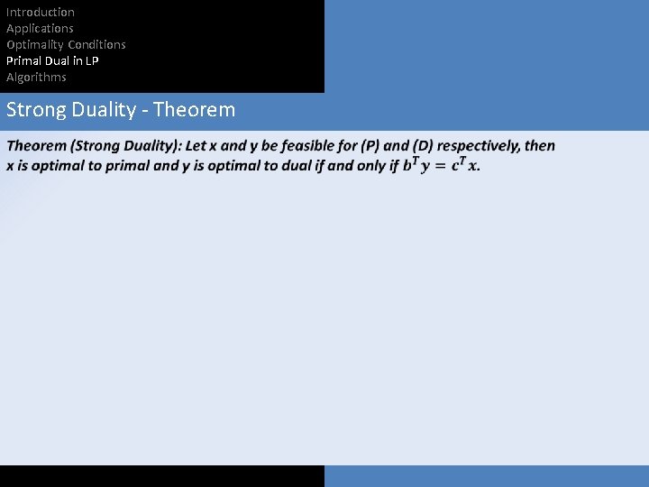
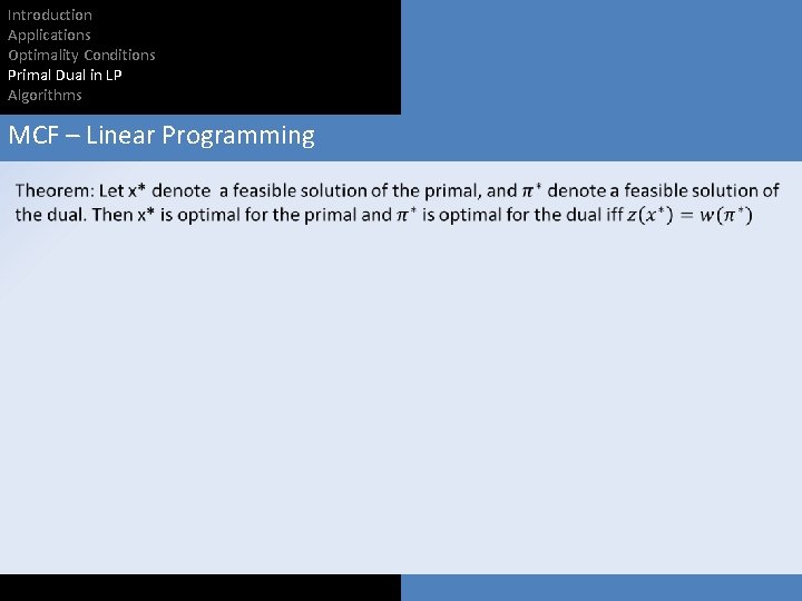
Introduction Applications Optimality Conditions Primal Dual in LP Algorithms Strong Duality - Theorem

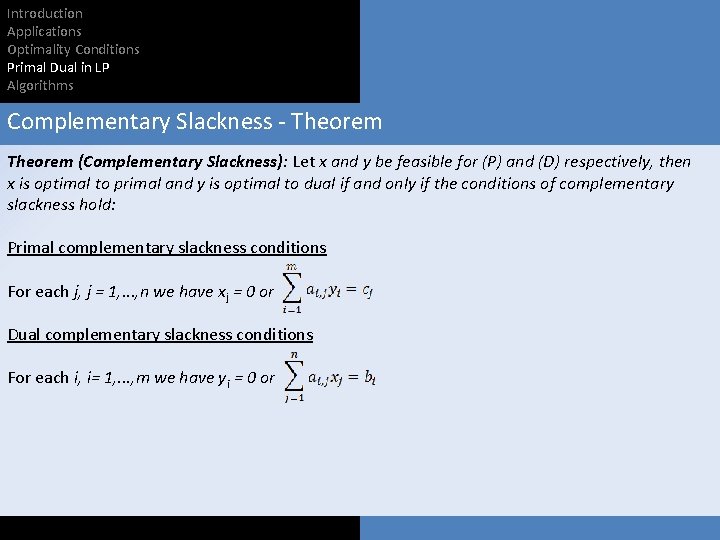
Introduction Applications Optimality Conditions Primal Dual in LP Algorithms Complementary Slackness - Theorem (Complementary Slackness): Let x and y be feasible for (P) and (D) respectively, then x is optimal to primal and y is optimal to dual if and only if the conditions of complementary slackness hold: Primal complementary slackness conditions For each j, j = 1, . . . , n we have xj = 0 or Dual complementary slackness conditions For each i, i= 1, . . . , m we have yi = 0 or

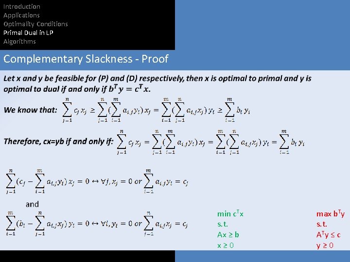
Introduction Applications Optimality Conditions Primal Dual in LP Algorithms Complementary Slackness - Proof min c. Tx s. t. Ax ≥ b x≥ 0 max b. Ty s. t. ATy ≤ c y≥ 0

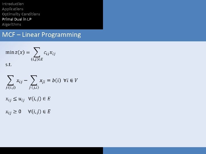
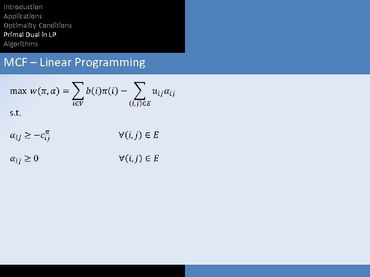
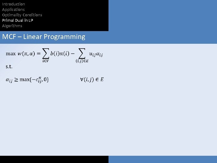
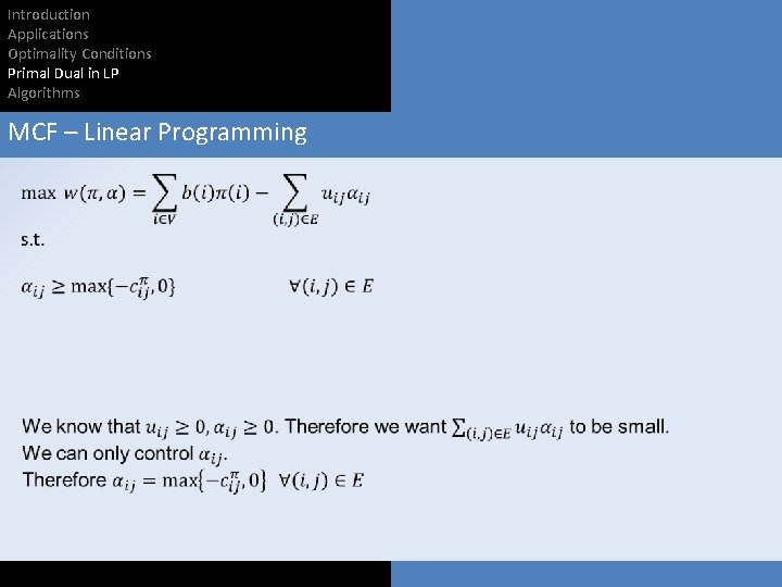
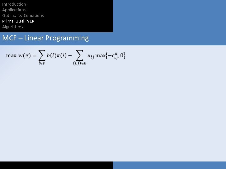
Introduction Applications Optimality Conditions Primal Dual in LP Algorithms MCF – Linear Programming

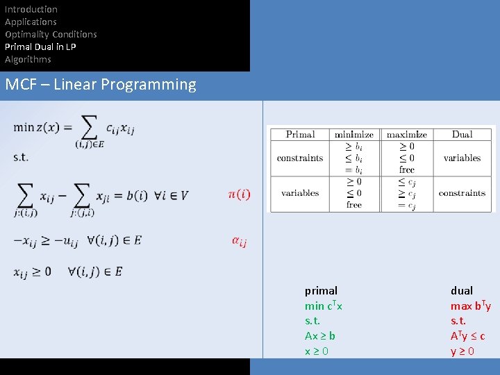
Introduction Applications Optimality Conditions Primal Dual in LP Algorithms MCF – Linear Programming primal min c. Tx s. t. Ax ≥ b x≥ 0 dual max b. Ty s. t. ATy ≤ c y≥ 0

Introduction Applications Optimality Conditions Primal Dual in LP Algorithms MCF – Linear Programming

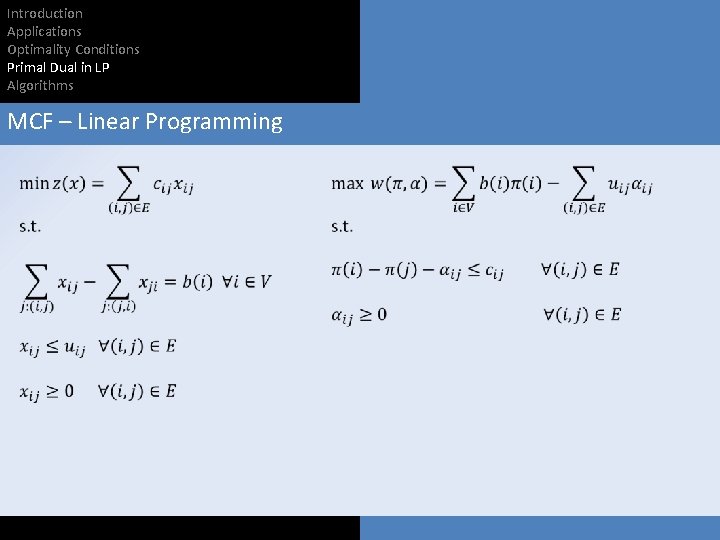
Introduction Applications Optimality Conditions Primal Dual in LP Algorithms MCF – Linear Programming

Introduction Applications Optimality Conditions Primal Dual in LP Algorithms MCF – Linear Programming

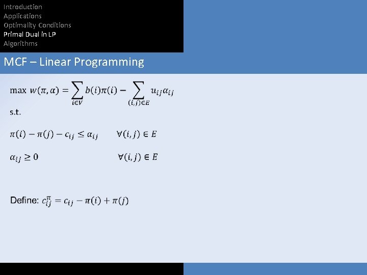
Introduction Applications Optimality Conditions Primal Dual in LP Algorithms MCF – Linear Programming

Introduction Applications Optimality Conditions Primal Dual in LP Algorithms MCF – Linear Programming

Introduction Applications Optimality Conditions Primal Dual in LP Algorithms MCF – Linear Programming

Introduction Applications Optimality Conditions Primal Dual in LP Algorithms MCF – Linear Programming

Introduction Applications Optimality Conditions Primal Dual in LP Algorithms MCF – Linear Programming

Introduction Applications Optimality Conditions Primal Dual in LP Algorithms MCF – Linear Programming Proof: Weak Duality Theorem.

Introduction Applications Optimality Conditions Primal Dual in LP Algorithms MCF – Linear Programming

Introduction Applications Optimality Conditions Primal Dual in LP Algorithms MCF – Linear Programming Proof: Strong Duality Theorem.

Introduction Applications Optimality Conditions Primal Dual in LP Algorithms MCF – Linear Programming

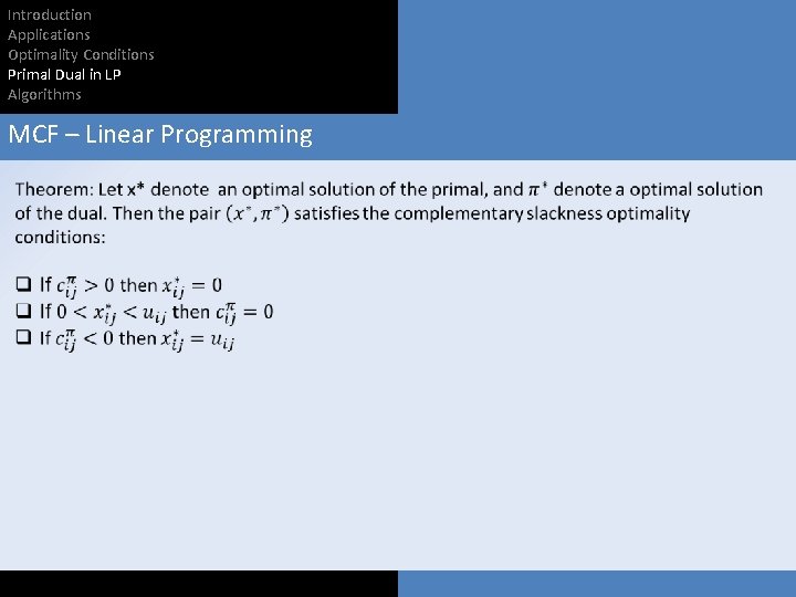
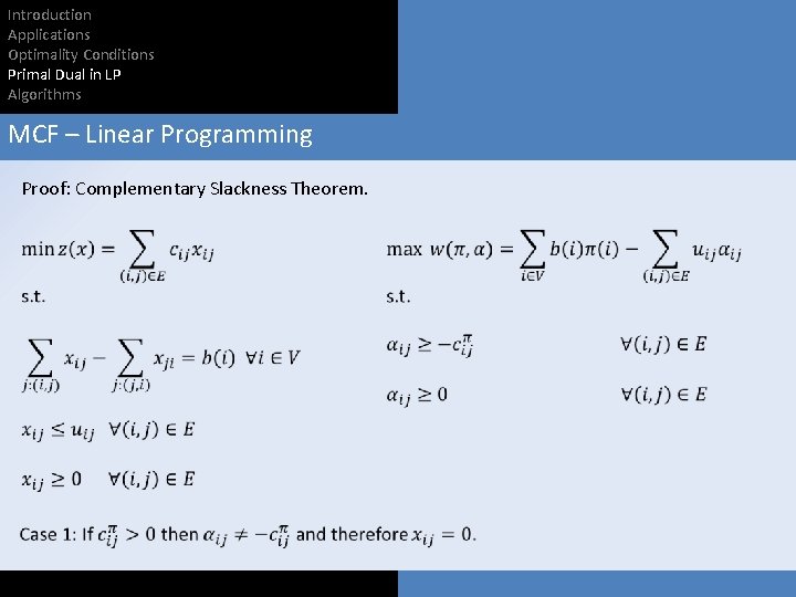
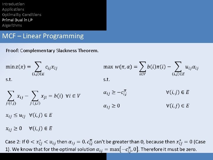
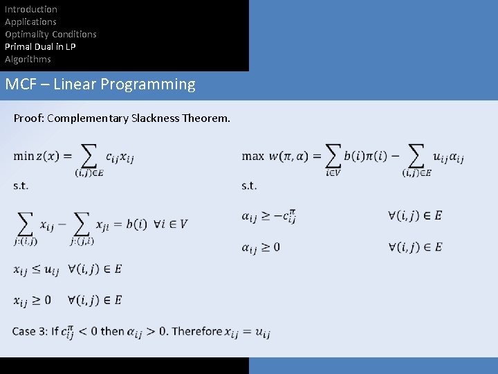
Introduction Applications Optimality Conditions Primal Dual in LP Algorithms MCF – Linear Programming Proof: Complementary Slackness Theorem.

Introduction Applications Optimality Conditions Primal Dual in LP Algorithms MCF – Linear Programming Proof: Complementary Slackness Theorem.

Introduction Applications Optimality Conditions Primal Dual in LP Algorithms MCF – Linear Programming Proof: Complementary Slackness Theorem.

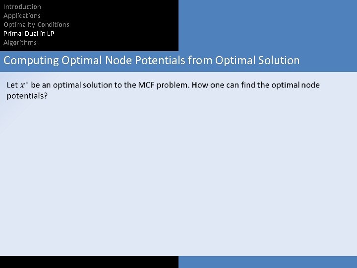
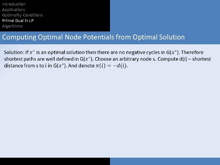
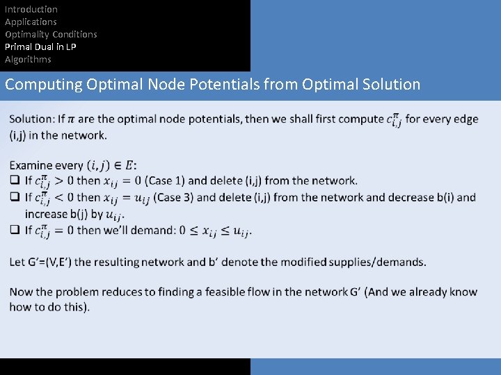
Introduction Applications Optimality Conditions Primal Dual in LP Algorithms Computing Optimal Node Potentials from Optimal Solution

Introduction Applications Optimality Conditions Primal Dual in LP Algorithms Computing Optimal Node Potentials from Optimal Solution

Introduction Applications Optimality Conditions Primal Dual in LP Algorithms Computing Optimal Flow from Optimal Node Potentials Given the optimal node potentials, how can one find the optimal flow?

Introduction Applications Optimality Conditions Primal Dual in LP Algorithms Computing Optimal Node Potentials from Optimal Solution

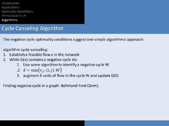
Introduction Applications Optimality Conditions Primal Dual in LP Algorithms Cycle Canceling Algorithm

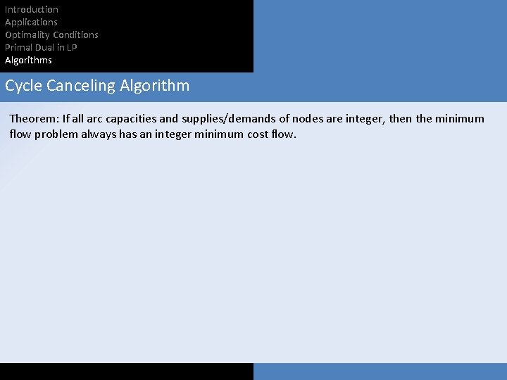
Introduction Applications Optimality Conditions Primal Dual in LP Algorithms Cycle Canceling Algorithm Theorem: If all arc capacities and supplies/demands of nodes are integer, then the minimum flow problem always has an integer minimum cost flow.

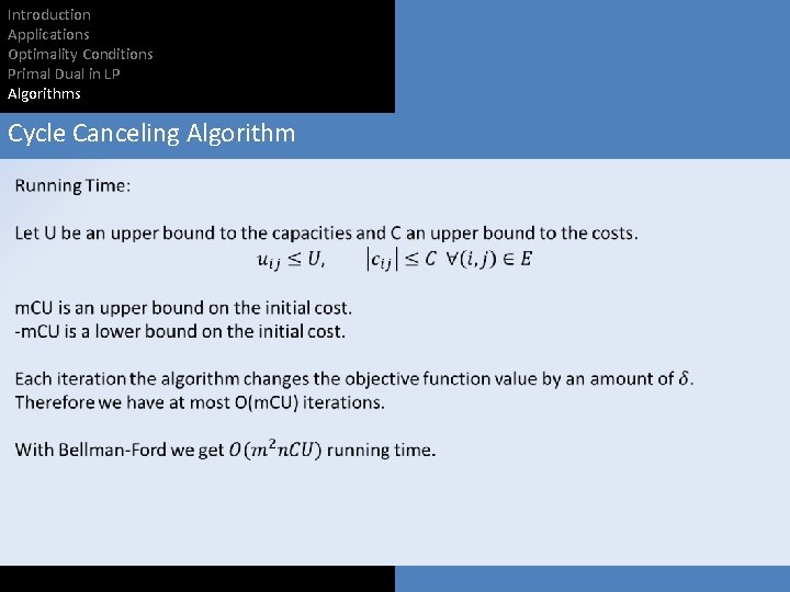
Introduction Applications Optimality Conditions Primal Dual in LP Algorithms Cycle Canceling Algorithm

Introduction Applications Optimality Conditions Primal Dual in LP Algorithms THANK YOU