Introduction and Descriptive Statistics WHAT IS STATISTICS STATISTICS

Introduction and Descriptive Statistics

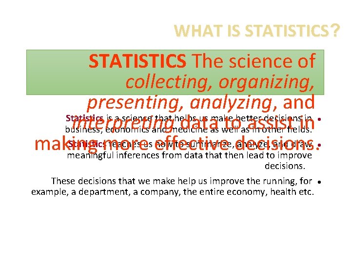
WHAT IS STATISTICS? STATISTICS The science of collecting, organizing, presenting, analyzing, and Statistics is a science that helps us make better decisions in interpreting dataas well toasassist in business, economics and medicine in other fields. Statisticsmore teaches us effective how to summarize, decisions. analyze, and draw making meaningful inferences from data that then lead to improve l l decisions. These decisions that we make help us improve the running, for l example, a department, a company, the entire economy, health etc.

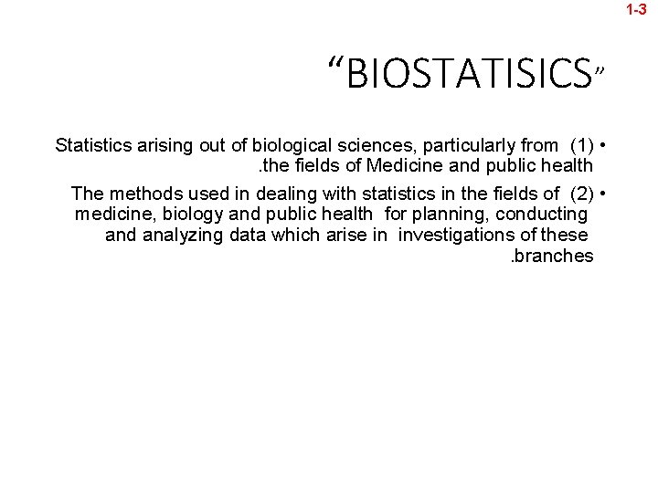
1 -3 “BIOSTATISICS” Statistics arising out of biological sciences, particularly from (1) • . the fields of Medicine and public health The methods used in dealing with statistics in the fields of (2) • medicine, biology and public health for planning, conducting and analyzing data which arise in investigations of these. branches

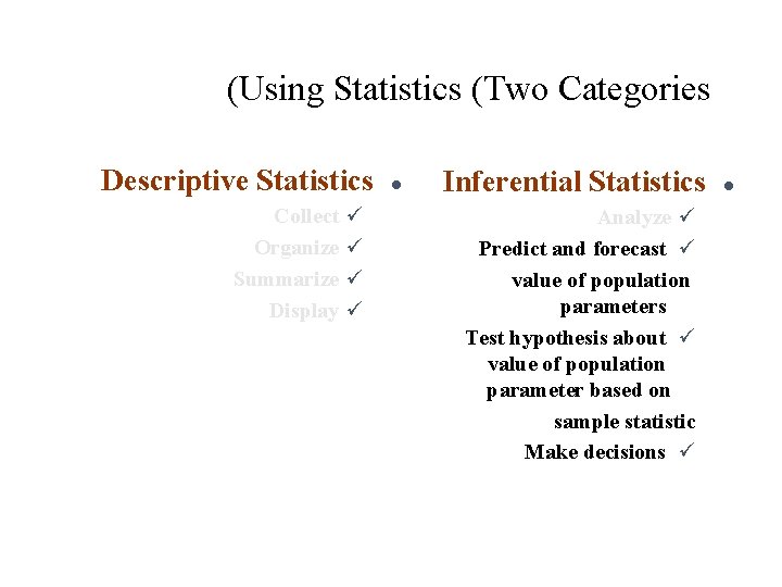
(Using Statistics (Two Categories Descriptive Statistics Collect Organize Summarize Display ü ü l Inferential Statistics Analyze ü Predict and forecast ü value of population parameters Test hypothesis about ü value of population parameter based on sample statistic Make decisions ü l

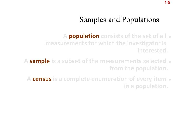
1 -5 Samples and Populations A population consists of the set of all l measurements for which the investigator is interested. A sample is a subset of the measurements selected l from the population. A census is a complete enumeration of every item l in a population.

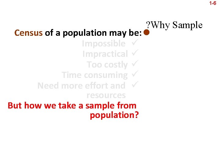
1 -6 ? Why Sample Census of a population may be: l Impossible ü Impractical ü Too costly ü Time consuming ü Need more effort and ü resources But how we take a sample from population?

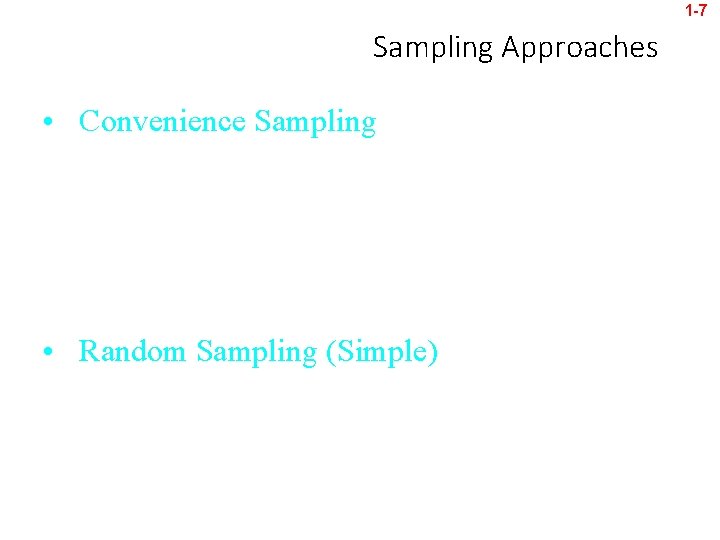
1 -7 Sampling Approaches • Convenience Sampling: select the most accessible and available subjects in target population. Inexpensive, less time consuming, but sample is nearly always non-representative of target population. • Random Sampling (Simple): select subjects at random from the target population. Need to identify all in target population first. Provides representative sample frequently. 7

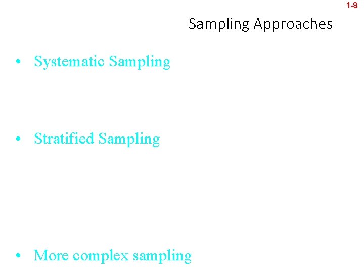
1 -8 Sampling Approaches • Systematic Sampling: Identify all in target population, and select every xth person as a subject. • Stratified Sampling: Identify important subgroups in your target population. Sample from these groups randomly or by convenience. Ensures that important sub-groups are included in sample. May not be representative. • More complex sampling 8

1 -9 Sampling Error The discrepancy between the true population parameter and the sample • statistic Sampling error likely exists in most studies, but can be reduced by using • larger sample sizes Sampling error approximates 1 / √n • Note that larger sample sizes also require time and expense to obtain, • and that large sample sizes do not eliminate sampling error 9

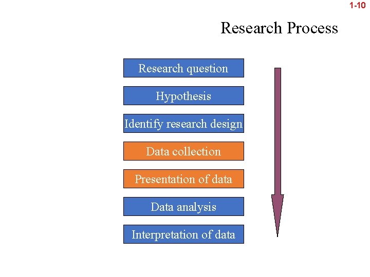
1 -10 Research Process Research question Hypothesis Identify research design Data collection Presentation of data Data analysis Interpretation of data 10

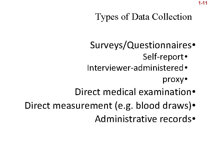
1 -11 Types of Data Collection Surveys/Questionnaires • Self-report • Interviewer-administered • proxy • Direct medical examination • Direct measurement (e. g. blood draws) • Administrative records • 11

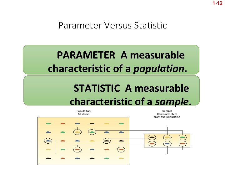
1 -12 Parameter Versus Statistic PARAMETER A measurable characteristic of a population. STATISTIC A measurable characteristic of a sample.

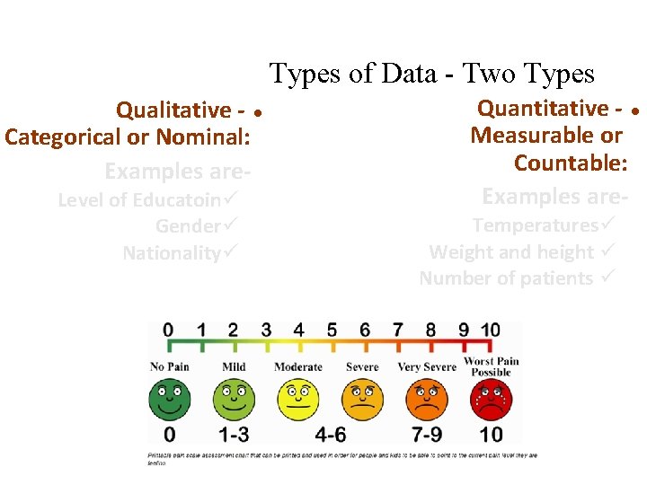
Types of Data - Two Types Qualitative - l Categorical or Nominal: Examples are. Level of Educatoinü Genderü Nationalityü Quantitative - l Measurable or Countable: Examples are. Temperaturesü Weight and height ü Number of patients ü

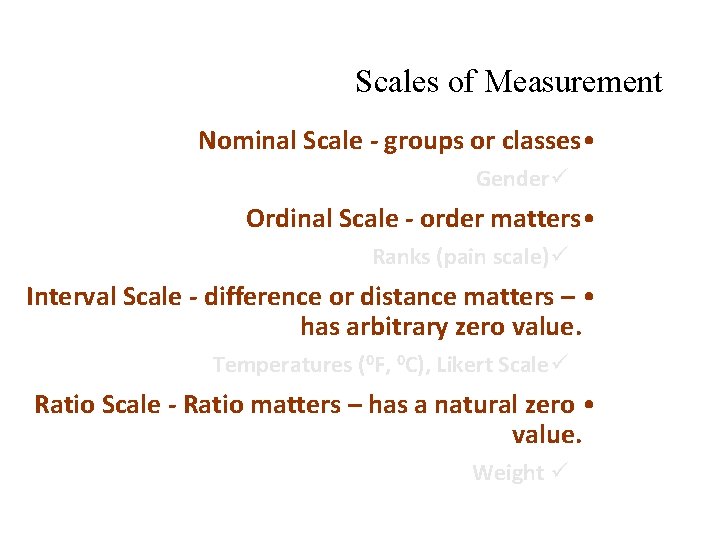
Scales of Measurement Nominal Scale - groups or classes • Genderü Ordinal Scale - order matters • Ranks (pain scale)ü Interval Scale - difference or distance matters – • has arbitrary zero value. Temperatures (0 F, 0 C), Likert Scaleü Ratio Scale - Ratio matters – has a natural zero • value. Weight ü

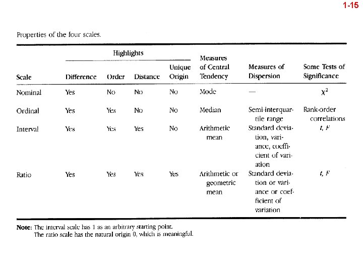
1 -15

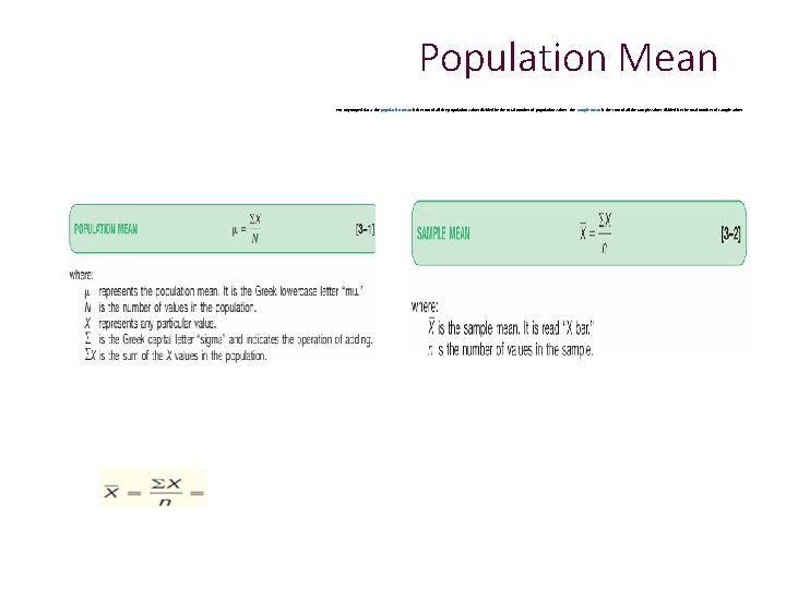
Population Mean For ungrouped data, the population mean is the sum of all the population values divided by the total number of population values. The sample mean is the sum of all the sample values divided by the total number of sample values. EXAMPLE: A random sample of size 10 of ages, where 1 = 42, 2 = 28, 3 = 28, 4 = 61, 5 = 31, 6 = 23, 7 = 50, 8 = 34, 9 = 32, 10 = 37. = (42 + 28 + … + 37) / 10 = 36. 6

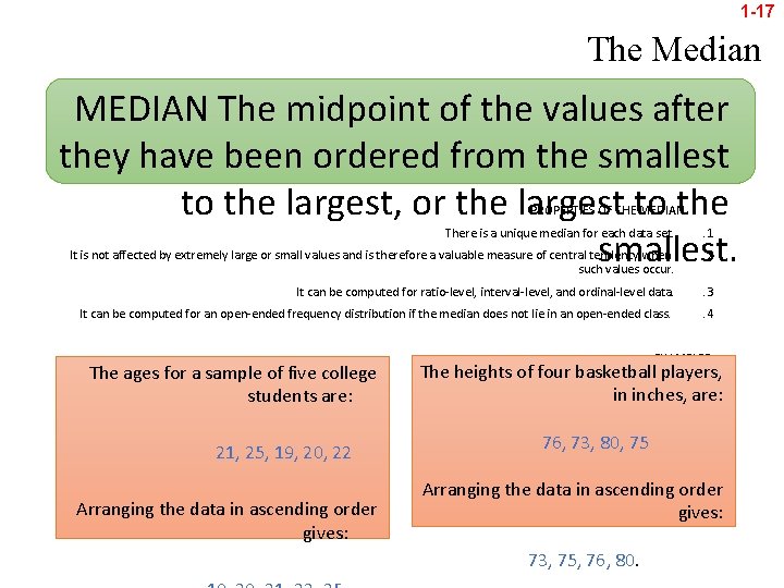
1 -17 The Median MEDIAN The midpoint of the values after they have been ordered from the smallest to the largest, or the largest to the smallest. PROPERTIES OF THE MEDIAN There is a unique median for each data set. . 1 It is not affected by extremely large or small values and is therefore a valuable measure of central tendency when such values occur. . 2 It can be computed for ratio-level, interval-level, and ordinal-level data. . 3 It can be computed for an open-ended frequency distribution if the median does not lie in an open-ended class. . 4 The ages for a sample of five college students are: 21, 25, 19, 20, 22 Arranging the data in ascending order gives: EXAMPLES: The heights of four basketball players, in inches, are: 76, 73, 80, 75 Arranging the data in ascending order gives: 73, 75, 76, 80.

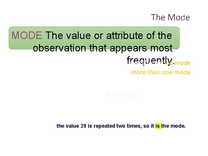
The Mode MODE The value or attribute of the observation that appears most If all valuesfrequently. are different no mode. Sometimes, there more than one mode. EXAMPLE: A random sample of size 10 of ages, where 1 = 42, 2 = 28, 3 = 28, 4 = 61, 5 = 31, 6 = 23, 7 = 50, 8 = 34, 9 = 32, 10 = 37. the value 28 is repeated two times, so it is the mode.

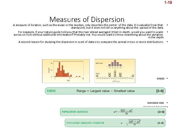
1 -19 Measures of Dispersion A measure of location, such as the mean or the median, only describes the center of the data. It is valuable from that • standpoint, but it does not tell us anything about the spread of the data. For example, if your nature guide told you that the river ahead averaged 3 feet in depth, would you want to wade • across on foot without additional information? Probably not. You would want to know something about the variation in the depth. A second reason for studying the dispersion in a set of data is to compare the spread in two or more distributions. • RANGE • VARIANCE AND • STANDARD DEVIATION

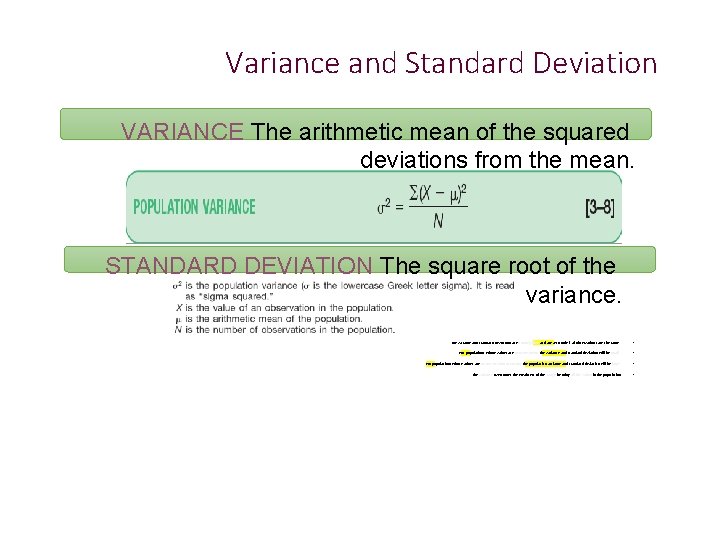
Variance and Standard Deviation VARIANCE The arithmetic mean of the squared deviations from the mean. STANDARD DEVIATION The square root of the variance. The variance and standard deviations are nonnegative and are zero only if all observations are the same. • For populations whose values are near the mean, the variance and standard deviation will be small. • For populations whose values are dispersed from the mean, the population variance and standard deviation will be large. • The variance overcomes the weakness of the range by using all the values in the population •

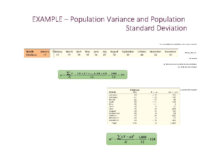
EXAMPLE – Population Variance and Population Standard Deviation The number of deadly traffic accidents during the last twelve months in one of region, is reported below: What is the population variance? Step 1: Find the mean. Step 2: Find the difference between each observation and the mean, and square that difference. Step 3: Sum all the squared differences found in step 3 Step 4: Divide the sum of the squared differences by the number of items in the population.

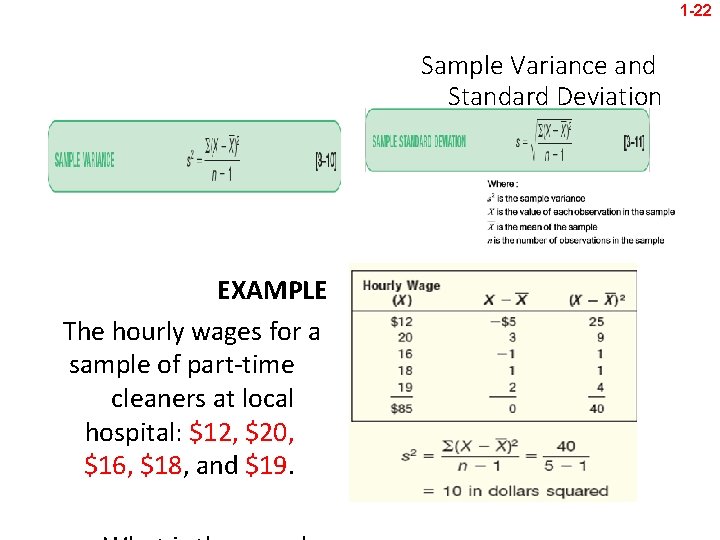
1 -22 Sample Variance and Standard Deviation EXAMPLE The hourly wages for a sample of part-time cleaners at local hospital: $12, $20, $16, $18, and $19.

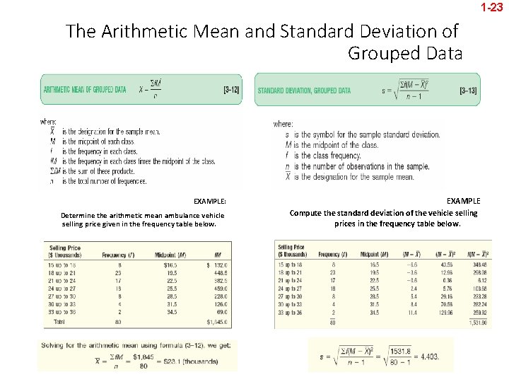
1 -23 The Arithmetic Mean and Standard Deviation of Grouped Data EXAMPLE: Determine the arithmetic mean ambulance vehicle selling price given in the frequency table below. EXAMPLE Compute the standard deviation of the vehicle selling prices in the frequency table below.

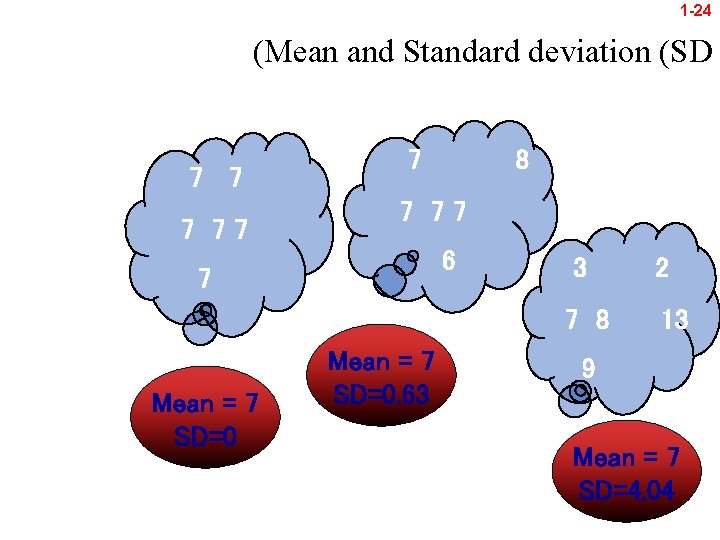
1 -24 (Mean and Standard deviation (SD 7 77 7 8 7 77 6 7 3 7 8 Mean = 7 SD=0. 63 2 13 9 Mean = 7 SD=4. 04 24

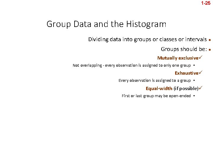
1 -25 Group Data and the Histogram Dividing data into groups or classes or intervals l Groups should be: l Mutually exclusiveü Not overlapping - every observation is assigned to only one group • Exhaustiveü Every observation is assigned to a group • Equal-width (if possible)ü First or last group may be open-ended •

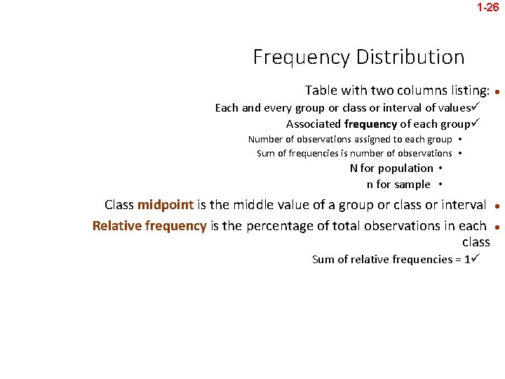
1 -26 Frequency Distribution Table with two columns listing: l Each and every group or class or interval of valuesü Associated frequency of each groupü Number of observations assigned to each group • Sum of frequencies is number of observations • N for population • n for sample • Class midpoint is the middle value of a group or class or interval l Relative frequency is the percentage of total observations in each l class Sum of relative frequencies = 1ü

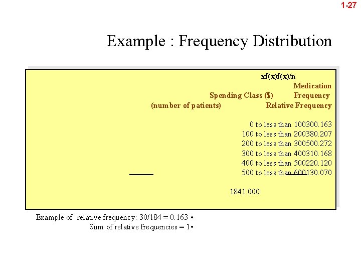
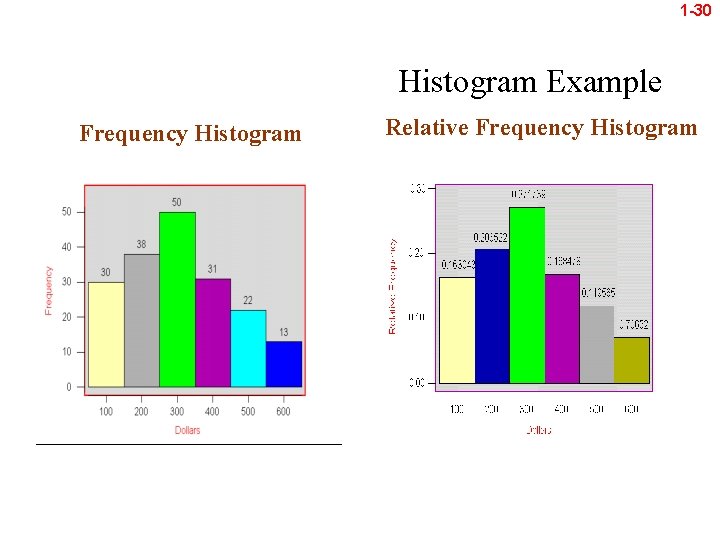
1 -27 Example : Frequency Distribution xf(x)/n Medication Spending Class ($) Frequency (number of patients) Relative Frequency 0 to less than 100300. 163 100 to less than 200380. 207 200 to less than 300500. 272 300 to less than 400310. 168 400 to less than 500220. 120 500 to less than 600130. 070 1841. 000 Example of relative frequency: 30/184 = 0. 163 • Sum of relative frequencies = 1 •

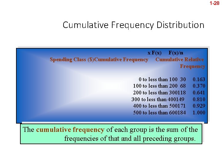
1 -28 Cumulative Frequency Distribution x F(x)/n Spending Class ($)Cumulative Frequency Cumulative Relative Frequency 0 to less than 100 30 100 to less than 200 68 200 to less than 300118 300 to less than 400149 400 to less than 500171 500 to less than 600184 0. 163 0. 370 0. 641 0. 810 0. 929 1. 000 The cumulative frequency of each group is the sum of the frequencies of that and all preceding groups.

1 -29 Histogram A histogram is a chart made of bars of different heights. l Widths and locations of bars correspond to widths and locations of data groupings ü Heights of bars correspond to frequencies or relative frequencies of data groupings ü

1 -30 Histogram Example Frequency Histogram Relative Frequency Histogram

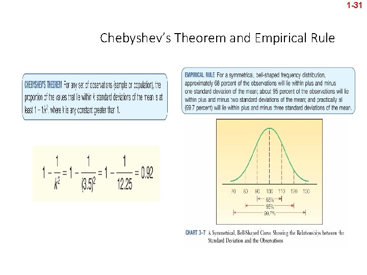
1 -31 Chebyshev’s Theorem and Empirical Rule

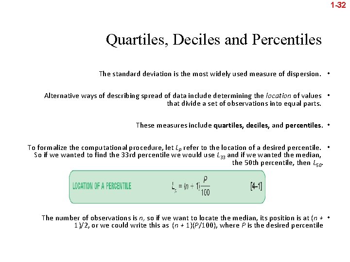
1 -32 Quartiles, Deciles and Percentiles The standard deviation is the most widely used measure of dispersion. • Alternative ways of describing spread of data include determining the location of values • that divide a set of observations into equal parts. These measures include quartiles, deciles, and percentiles. • To formalize the computational procedure, let Lp refer to the location of a desired percentile. • So if we wanted to find the 33 rd percentile we would use L 33 and if we wanted the median, the 50 th percentile, then L 50. The number of observations is n, so if we want to locate the median, its position is at (n + • 1)/2, or we could write this as (n + 1)(P/100), where P is the desired percentile

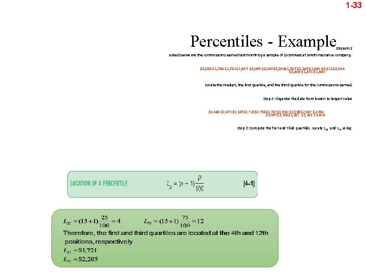
1 -33 Percentiles - Example EXAMPLE Listed below are the commissions earned last month by a sample of 15 brokers at Smith insurance company. $2, 038 $1, 758 $1, 721 $1, 637 $2, 097 $2, 047 $2, 205$1, 787 $2, 287 $1, 940 $2, 311 $2, 054 $2, 406 $1, 471 $1, 460 Locate the median, the first quartile, and the third quartile for the commissions earned. Step 1: Organize the data from lowest to largest value $1, 460 $1, 471 $1, 637$1, 721$1, 758$1, 787$1, 940 $2, 038$2, 047 $2, 054 $2, 097$2, 205$2, 287 $2, 311 $2, 406 Step 2: Compute the first and third quartiles. Locate L 25 and L 75 using:

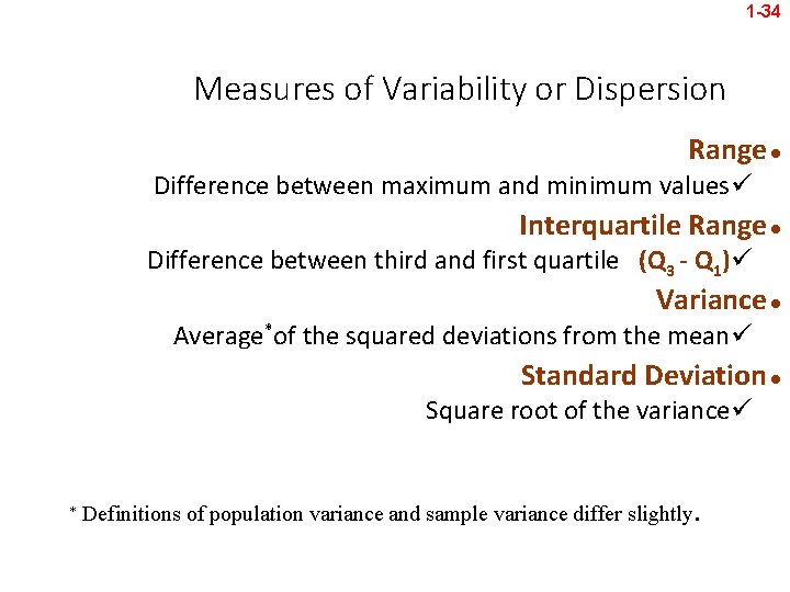
1 -34 Measures of Variability or Dispersion Range l Difference between maximum and minimum valuesü Interquartile Range l Difference between third and first quartile (Q 3 - Q 1)ü Variance l Average*of the squared deviations from the meanü Standard Deviation l Square root of the varianceü Definitions of population variance and sample variance differ slightly .

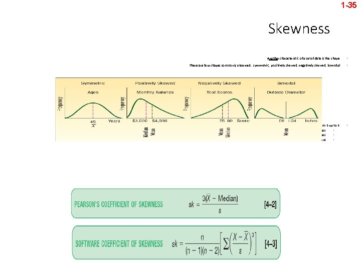
1 -35 Skewness Another characteristic of a set of data is the shape. • There are four shapes commonly observed: symmetric, positively skewed, negatively skewed, bimodal. • The coefficient of skewness can range from -3 up to 3. A value near -3, indicates considerable negative skewness. • A value such as 1. 63 indicates moderate positive skewness. • A value of 0, which will occur when the mean and median are equal, indicates the distribution is symmetrical and that there is no skewness present. • •

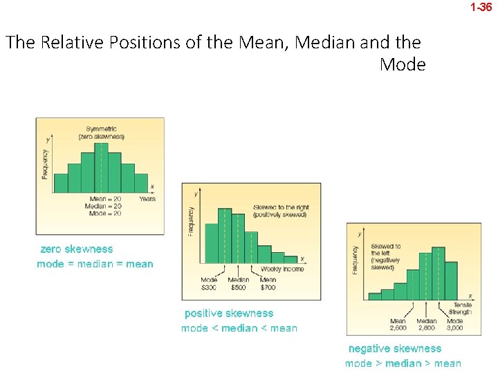
1 -36 The Relative Positions of the Mean, Median and the Mode

Methods of Displaying Data Pie Charts l Categories represented as percentages of totalü Bar Graphs l Heights of rectangles represent group frequenciesü Frequency Polygons l Height of line represents frequency ü Ogives l Height of line represents cumulative frequencyü Time Series Plots l Represents values over timeü Stem-and-Leaf Displays • Quick listing of all observations ü Conveys some of the same information as a histogramü Box Plots • Medianü Lower and upper quartilesü Maximum and minimumü

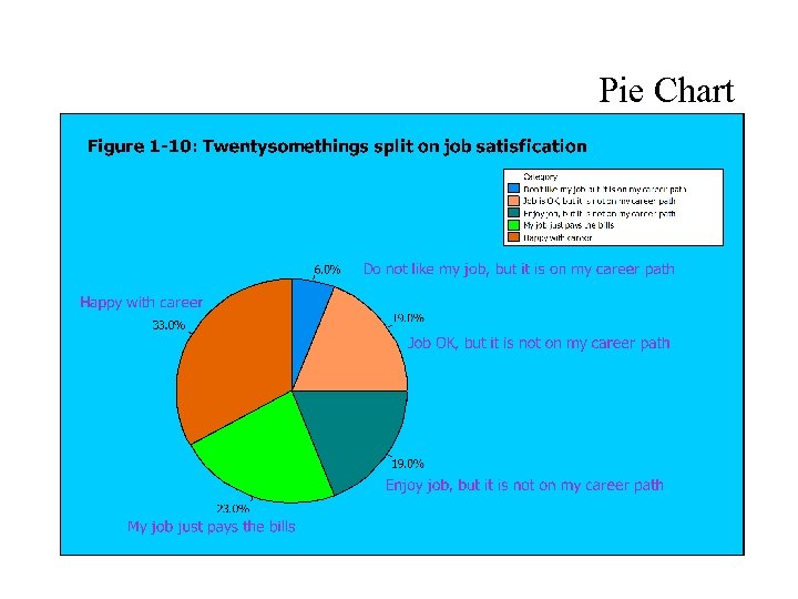
Pie Chart

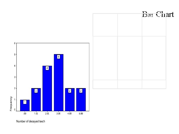
Bar Chart Relative No. of decayed teeth Frequency 0 1 2 3 4 5 1 2 4 5 2 2 0. 0625 0. 125 0. 3125 0. 125 Total 16 1 Frequency

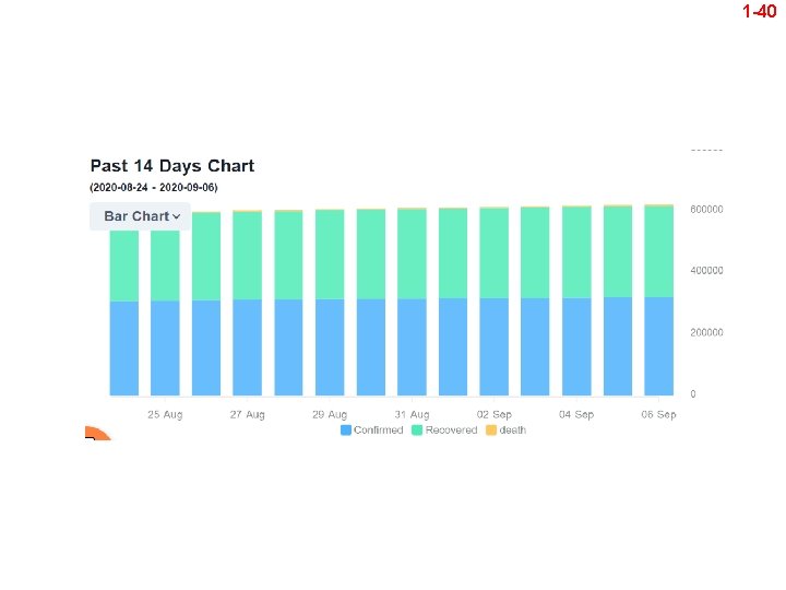
1 -40

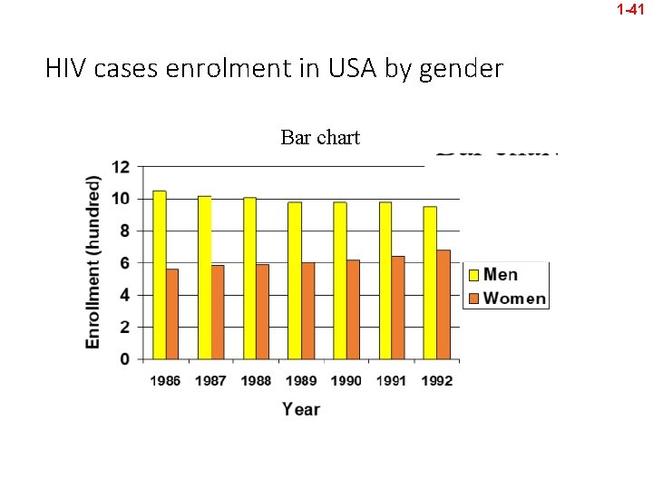
1 -41 HIV cases enrolment in USA by gender Bar chart

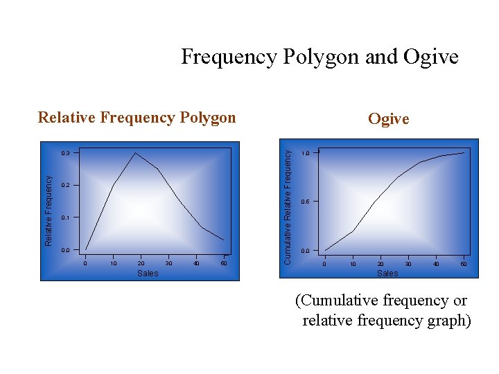
Frequency Polygon and Ogive Relative Frequency Polygon 0. 2 0. 1 0. 0 0 10 20 Sales 30 40 50 Cumulative Relative Frequency 0. 3 Ogive 1. 0 0. 5 0. 0 0 10 20 30 40 50 Sales (Cumulative frequency or relative frequency graph)

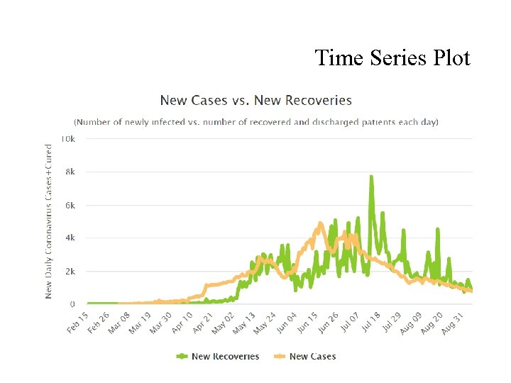
Time Series Plot

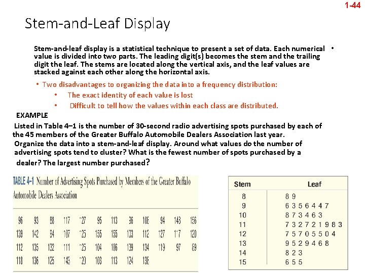
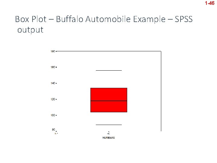
1 -44 Stem-and-Leaf Display Stem-and-leaf display is a statistical technique to present a set of data. Each numerical • value is divided into two parts. The leading digit(s) becomes the stem and the trailing digit the leaf. The stems are located along the vertical axis, and the leaf values are stacked against each other along the horizontal axis. • Two disadvantages to organizing the data into a frequency distribution: • The exact identity of each value is lost • Difficult to tell how the values within each class are distributed. EXAMPLE Listed in Table 4– 1 is the number of 30 -second radio advertising spots purchased by each of the 45 members of the Greater Buffalo Automobile Dealers Association last year. Organize the data into a stem-and-leaf display. Around what values do the number of advertising spots tend to cluster? What is the fewest number of spots purchased by a dealer? The largest number purchased?

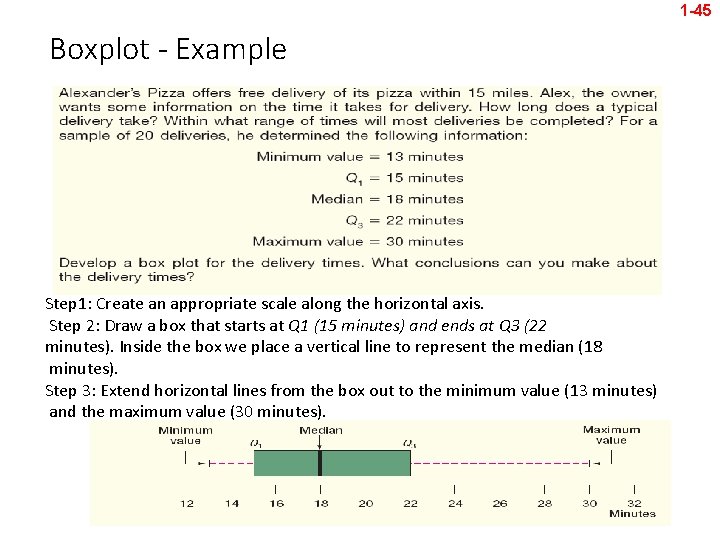
1 -45 Boxplot - Example Step 1: Create an appropriate scale along the horizontal axis. Step 2: Draw a box that starts at Q 1 (15 minutes) and ends at Q 3 (22 minutes). Inside the box we place a vertical line to represent the median (18 minutes). Step 3: Extend horizontal lines from the box out to the minimum value (13 minutes) and the maximum value (30 minutes).

1 -46 Box Plot – Buffalo Automobile Example – SPSS output

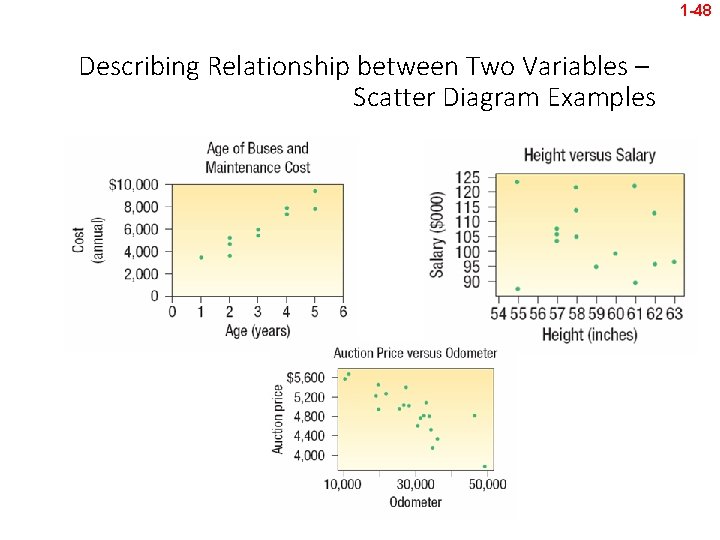
Scatter Plots are used to identify and report • any underlying relationships among pairs of data sets. The plot consists of a scatter of points, each • point representing an observation.

1 -48 Describing Relationship between Two Variables – Scatter Diagram Examples

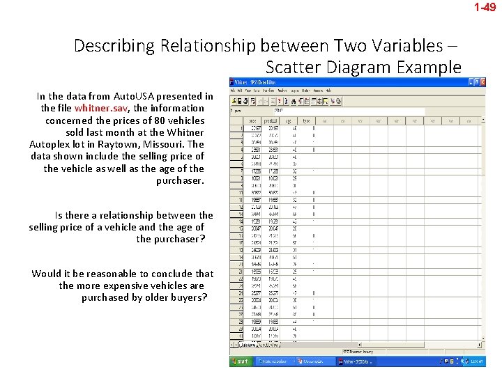
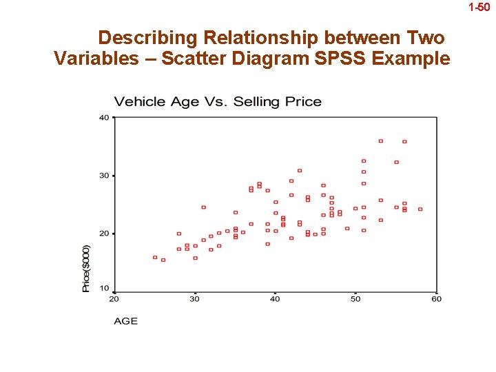
1 -49 Describing Relationship between Two Variables – Scatter Diagram Example In the data from Auto. USA presented in the file whitner. sav, the information concerned the prices of 80 vehicles sold last month at the Whitner Autoplex lot in Raytown, Missouri. The data shown include the selling price of the vehicle as well as the age of the purchaser. Is there a relationship between the selling price of a vehicle and the age of the purchaser? Would it be reasonable to conclude that the more expensive vehicles are purchased by older buyers?

1 -50 Describing Relationship between Two Variables – Scatter Diagram SPSS Example