INTRODUCTI ON A graph GV E consists of

INTRODUCTI ON A graph G=(V, E) consists of a finite non empty set of vertices V , and a finite set of edges E which connect pairs of vertices. V={1, 2, 3, 4, 5} E={(1, 4) , (4, 2) , (2, 5) , (3, 5) , (4, 5)}

TERMINOLOGIES Multigraph : A multigraph G=(V, E) consists of a set of vertices and edges and E may contain multiple edges , i. e. , edges containing the same pair of vertices or self edges. Directed Graph : A directed graph is one in which each edge is an ordered pair of vertices. i. e. (v 1, v 2) !=(v 2, v 1)

Undirected Graph : A graph whose definition makes reference to unordered pairs of vertices. i. e. (v 1, v 2)=(v 2, v 1).

Degree : Degree of a vertex is the number of edges incident to that vertex. In case of directed graphs, number of edges going into a node is known as in degree of the corresponding node and number of edges coming out of a node is known as outdegree of the corresponding node. For e. g. degree of vertex 2 is 2 in the above example and degree of vertex 5 is 3. Complete graphs : An undirected graph with n vertices and n. C 2 edges is said to be complete.

Subgraph : A subgraph G’={V’, E’} of a graph G is such that V’ is a subset of V and E’ is a subset of E. Path : A path from vertex V 1 to Vk in an undirected graph G is a sequence of vertices V 1, V 2, . . . Vk such that consecutive Vi and Vi+1 are adjacent. Cycle : When the first and last vertex is same in a path. Connected graphs : An undirected graph is said to be a connected graph if every pair of distinct vertices Vi , Vj are connected.

REPRESENTATION OF GRAPHS 1. Adjacency Matrix : The adjacency matrix of a graph G=(V, E) is a two dimensional V by V array , say A such that : If the edge (vi, vj) is in E , A[i][j]=1 If the edge (vi, vj) is not present , A[i][j]=0 The adjacency matrix for an undirected graph is symmetric.

2. Adjacency List : Each row of an adjacency matrix is represented as an adjacency list.

SPANNING TREES A subgraph T of an undirected graph G=(V, E) is a spanning tree of G if it is a tree and contains every vertex of G.

WEIGHTED GRAPHS A weighted graph is a graph in which each edge has a weight.

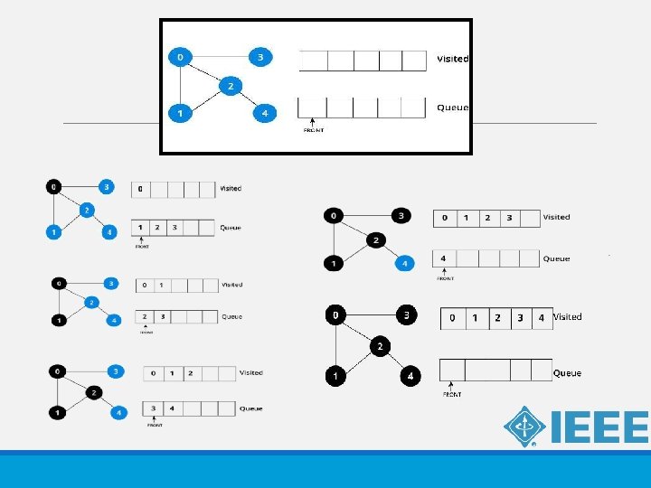
BFS is a traversing algorithm where you should start traversing from a selected node (source or starting node) and traverse the graph layerwise thus exploring the neighbour nodes (nodes which are directly connected to source node).

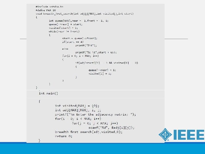
ALGORITHM Create an empty queue and a visited array initialized as false for each vertex. Select the source vertex. 1. Create a queue and enqueue the source into it. 2. Mark the source as visited. 3. While the queue is not empty, do the following 3 a. Dequeue a vertex from the queue, let’s call this temp. 3 b. Print temp. 3 c. Enqueue all not yet visited adjacent vertices of temp and mark them visited.

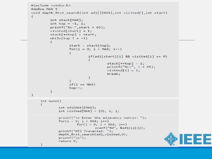
DFS The strategy followed by depth-first search is, as its name implies, to search “deeper” in the graph whenever possible. In depth-first search, edges are explored out of the most recently discovered vertex v that still has unexplored edges leaving it. When all of v’s edges have been explored, the search “backtracks” to explore edges leaving the vertex from which v was discovered. This process continues until we have discovered all the vertices that are reachable from the original source vertex. If any undiscovered vertices remain, then one of them is selected as a new source and the search is repeated from that source. This entire process is repeated until all vertices are discovered.

ALGORITHM Create an empty stack and a visited array initialized as zero for each vertex. 1. Push the source vertex in the stack. 2. While stack is not empty, do the following: 2 a. Pop an element from stack, let’s call it u 2 b. If u has not been visited then Set visited of u as true. For each unvisited adjacent vertex of u, push it into the stack.

N

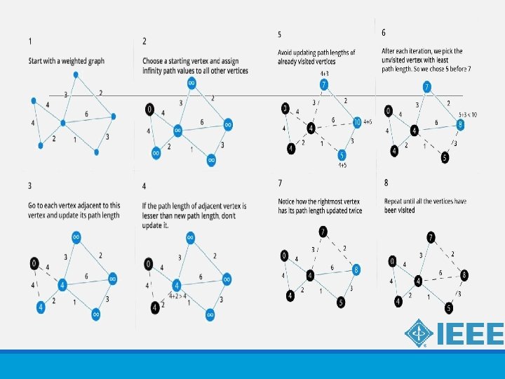
DIJKSTRA’S ALGORITHM 1) Create a set spt. Set(shortest path tree set) that keeps track of vertices included in shortest path tree, i. e. , whose minimum distance from source is calculated and finalized. Initially, this set is empty. 2) Assign a distance value to all vertices in the input graph. Initialize all distance values as INFINITE. Assign distance value as 0 for the source vertex so that it is picked first. 3)While spt. Setdoesn’t include all vertices …. a)Pick a vertex u which is not there in spt. Set and has minimum distance value. …. b)Include u to spt. Set. …. c)Update distance value of all adjacent vertices of u. To update the distance values, iterate through all adjacent vertices. For every adjacent vertex v, if sum of distance value of u (from source) and weight of edge u-v, is less than the distance value of v, then update the distance value of v. Time compexity : The time complexity for the following algorithm is O(|E| + |V|^2)

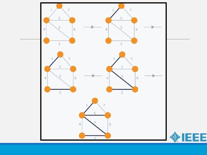
KRUSKAL’S ALGORITHM Kruskal’s Algorithm builds the spanning tree by adding edges one by one into a growing spanning tree. Kruskal's algorithm follows greedy approach as in each iteration it finds an edge which has least weight and add it to the growing spanning tree.

ALGORITHM STEPS ● Sort the graph edges with respect to their weights. ● Start adding edges to the MST from the edge with the smallest weight until the edge of the largest weight. ● Only add edges which doesn't form a cycle , edges which connect only disconnected components. Kruskal's algorithm can be shown to run in O(E log E ) time, or equivalently, O(E log V) time, where E is the number of edges in the graph and V is the number of vertices.

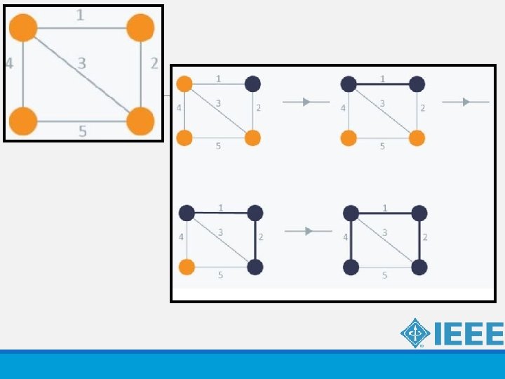
PRIM’S ALGORITHM Prim’s Algorithm also use Greedy approach to find the minimum spanning tree. In Prim’s Algorithm we grow the spanning tree from a starting position. Unlike an edge in Kruskal's, we add vertex to the growing spanning tree in Prim's.

ALGORITHM STEPS ● Maintain two disjoint sets of vertices. One containing vertices that are in the growing spanning tree and other that are not in the growing spanning tree. ● Select the cheapest vertex that is connected to the growing spanning tree and is not in the growing spanning tree and add it into the growing spanning tree. This can be done using Priority Queues. Insert the vertices, that are connected to growing spanning tree, into the Priority Queue. ● Check for cycles. To do that, mark the nodes which have been already selected and insert only those nodes in the Priority Queue that are not marked. The time complexity is O(Vlog. V + Elog. V) = O(Elog. V), making it the same as Kruskal’s algorithm.