Intro to Statistics Part II Descriptive Statistics Ernesto

Intro to Statistics Part II Descriptive Statistics Ernesto Diaz Assistant Professor of Mathematics Copyright © 2016 Brooks/Cole Cengage Learning

14. 2 Descriptive Statistics Copyright © Cengage Learning. All rights reserved.

Descriptive Statistics Descriptive statistics is concerned with the accumulation of data, measures of central tendency, and dispersion. 3

Measures of Central Tendency 4

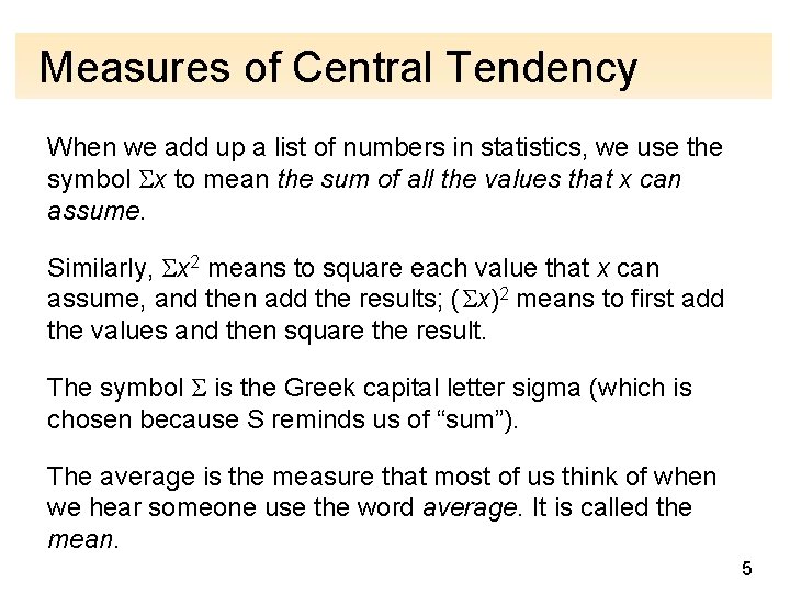
Measures of Central Tendency When we add up a list of numbers in statistics, we use the symbol x to mean the sum of all the values that x can assume. Similarly, x 2 means to square each value that x can assume, and then add the results; ( x)2 means to first add the values and then square the result. The symbol is the Greek capital letter sigma (which is chosen because S reminds us of “sum”). The average is the measure that most of us think of when we hear someone use the word average. It is called the mean. 5

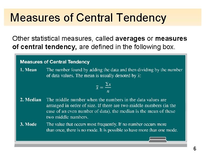
Measures of Central Tendency Other statistical measures, called averages or measures of central tendency, are defined in the following box. 6

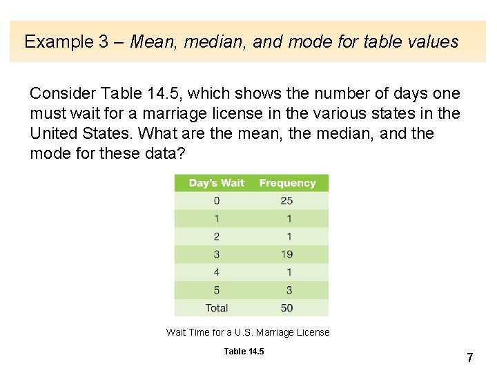
Example 3 – Mean, median, and mode for table values Consider Table 14. 5, which shows the number of days one must wait for a marriage license in the various states in the United States. What are the mean, the median, and the mode for these data? Wait Time for a U. S. Marriage License Table 14. 5 7

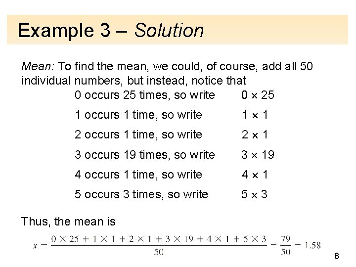
Example 3 – Solution Mean: To find the mean, we could, of course, add all 50 individual numbers, but instead, notice that 0 occurs 25 times, so write 0 25 1 occurs 1 time, so write 1 1 2 occurs 1 time, so write 2 1 3 occurs 19 times, so write 3 19 4 occurs 1 time, so write 4 1 5 occurs 3 times, so write 5 3 Thus, the mean is 8

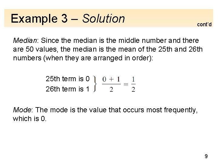
Example 3 – Solution cont’d Median: Since the median is the middle number and there are 50 values, the median is the mean of the 25 th and 26 th numbers (when they are arranged in order): 25 th term is 0 26 th term is 1 Mode: The mode is the value that occurs most frequently, which is 0. 9

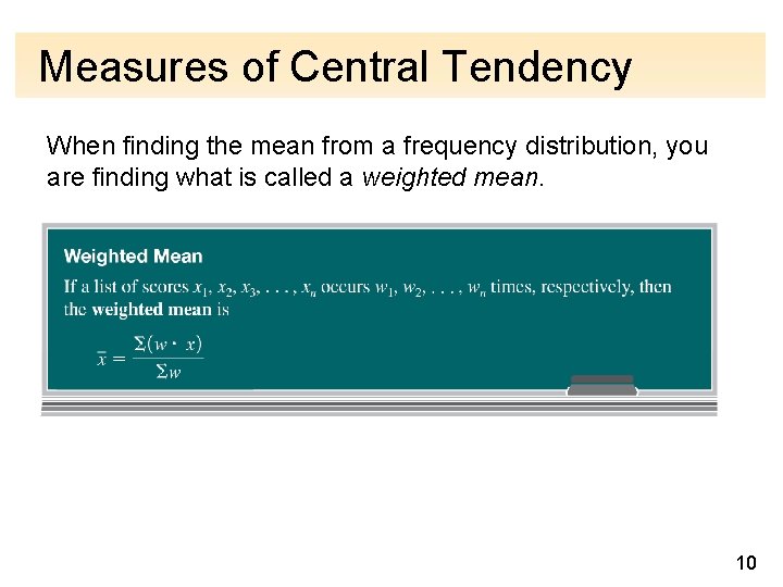
Measures of Central Tendency When finding the mean from a frequency distribution, you are finding what is called a weighted mean. 10

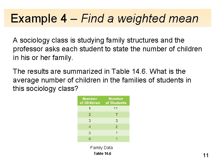
Example 4 – Find a weighted mean A sociology class is studying family structures and the professor asks each student to state the number of children in his or her family. The results are summarized in Table 14. 6. What is the average number of children in the families of students in this sociology class? Family Data Table 14. 6 11

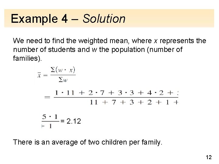
Example 4 – Solution We need to find the weighted mean, where x represents the number of students and w the population (number of families). = 2. 12 There is an average of two children per family. 12

Measures of Position 13

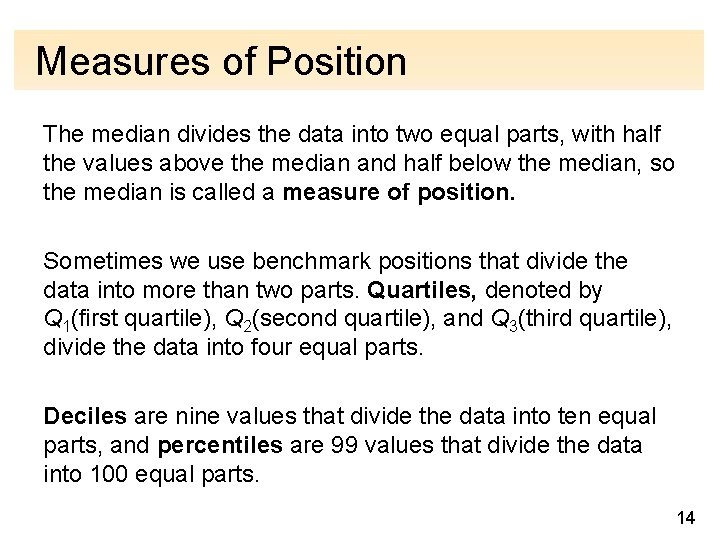
Measures of Position The median divides the data into two equal parts, with half the values above the median and half below the median, so the median is called a measure of position. Sometimes we use benchmark positions that divide the data into more than two parts. Quartiles, denoted by Q 1(first quartile), Q 2(second quartile), and Q 3(third quartile), divide the data into four equal parts. Deciles are nine values that divide the data into ten equal parts, and percentiles are 99 values that divide the data into 100 equal parts. 14

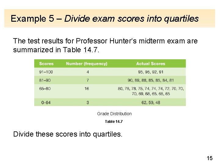
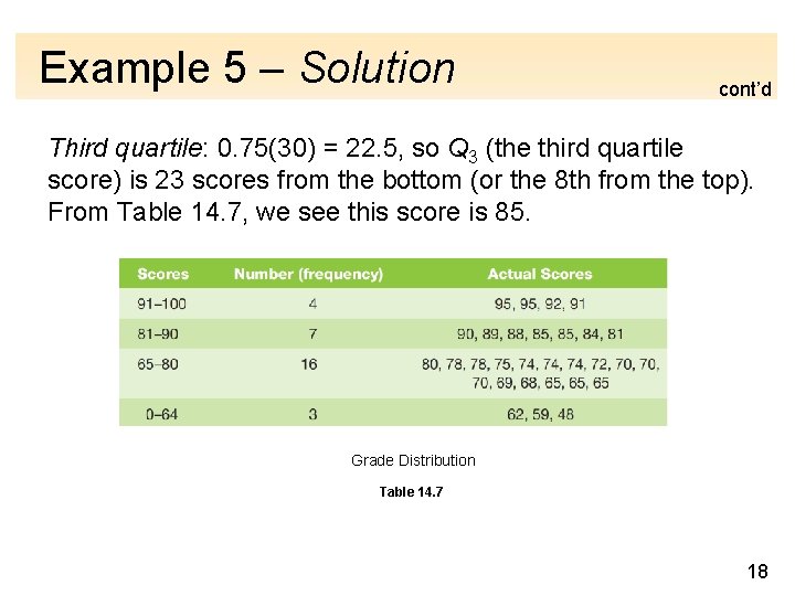
Example 5 – Divide exam scores into quartiles The test results for Professor Hunter’s midterm exam are summarized in Table 14. 7. Grade Distribution Table 14. 7 Divide these scores into quartiles. 15

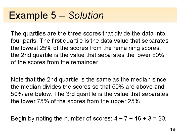
Example 5 – Solution The quartiles are three scores that divide the data into four parts. The first quartile is the data value that separates the lowest 25% of the scores from the remaining scores; the 2 nd quartile is the value that separates the lower 50% of the scores from the remainder. Note that the 2 nd quartile is the same as the median since the median divides the scores so that 50% are above and 50% are below. The 3 rd quartile is the value that separates the lower 75% of the scores from the upper 25%. Begin by noting the number of scores: 4 + 7 + 16 + 3 = 30. 16

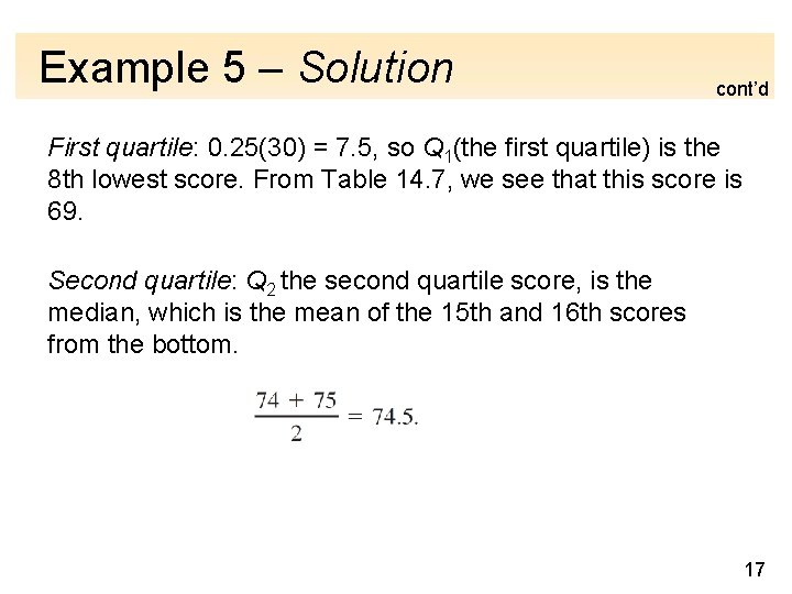
Example 5 – Solution cont’d First quartile: 0. 25(30) = 7. 5, so Q 1(the first quartile) is the 8 th lowest score. From Table 14. 7, we see that this score is 69. Second quartile: Q 2 the second quartile score, is the median, which is the mean of the 15 th and 16 th scores from the bottom. 17

Example 5 – Solution cont’d Third quartile: 0. 75(30) = 22. 5, so Q 3 (the third quartile score) is 23 scores from the bottom (or the 8 th from the top). From Table 14. 7, we see this score is 85. Grade Distribution Table 14. 7 18

Measures of Dispersion 19

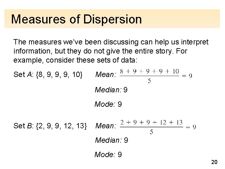
Measures of Dispersion The measures we’ve been discussing can help us interpret information, but they do not give the entire story. For example, consider these sets of data: Set A: {8, 9, 9, 9, 10} Mean: Median: 9 Mode: 9 Set B: {2, 9, 9, 12, 13} Mean: Median: 9 Mode: 9 20

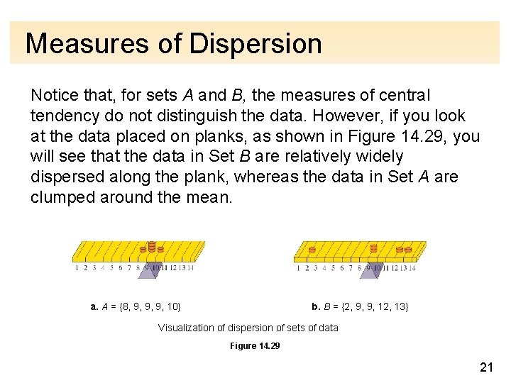
Measures of Dispersion Notice that, for sets A and B, the measures of central tendency do not distinguish the data. However, if you look at the data placed on planks, as shown in Figure 14. 29, you will see that the data in Set B are relatively widely dispersed along the plank, whereas the data in Set A are clumped around the mean. a. A = {8, 9, 9, 9, 10} b. B = {2, 9, 9, 12, 13} Visualization of dispersion of sets of data Figure 14. 29 21

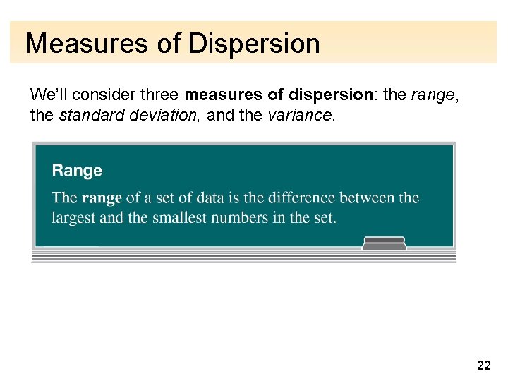
Measures of Dispersion We’ll consider three measures of dispersion: the range, the standard deviation, and the variance. 22

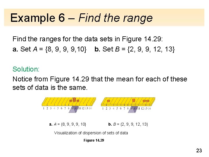
Example 6 – Find the ranges for the data sets in Figure 14. 29: a. Set A = {8, 9, 9, 9, 10} b. Set B = {2, 9, 9, 12, 13} Solution: Notice from Figure 14. 29 that the mean for each of these sets of data is the same. a. A = {8, 9, 9, 9, 10} b. B = {2, 9, 9, 12, 13} Visualization of dispersion of sets of data Figure 14. 29 23

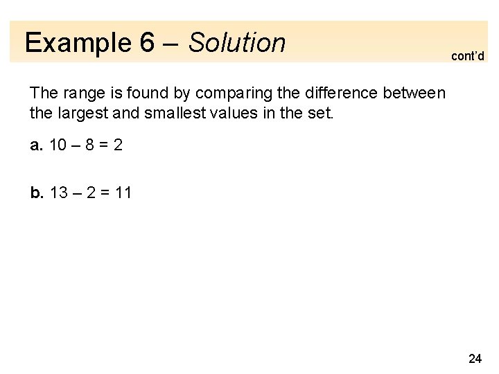
Example 6 – Solution cont’d The range is found by comparing the difference between the largest and smallest values in the set. a. 10 – 8 = 2 b. 13 – 2 = 11 24

Measures of Dispersion The range is used, along with quartiles, to construct a statistical tool called a box plot. For a given set of data, a box plot consists of a rectangular box positioned above a numerical scale, drawn from Q 1 (the first quartile) to Q 3 (the third quartile). The median ( Q 2, or second quartile) is shown as a dashed line, and a segment is extended to the left to show the distance to the minimum value; another segment is extended to the right for the maximum value. 25

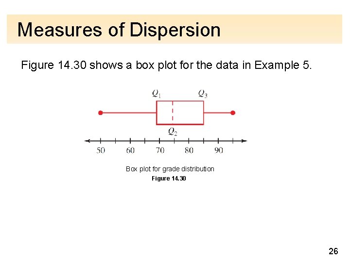
Measures of Dispersion Figure 14. 30 shows a box plot for the data in Example 5. Box plot for grade distribution Figure 14. 30 26

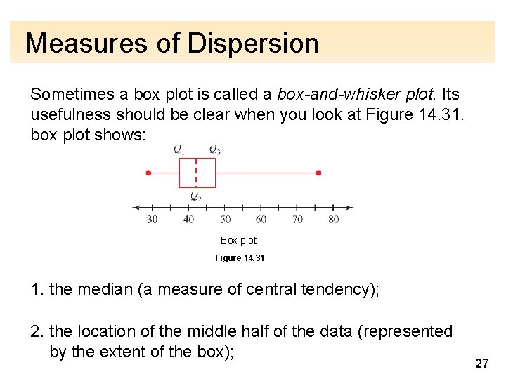
Measures of Dispersion Sometimes a box plot is called a box-and-whisker plot. Its usefulness should be clear when you look at Figure 14. 31. box plot shows: Box plot Figure 14. 31 1. the median (a measure of central tendency); 2. the location of the middle half of the data (represented by the extent of the box); 27

Measures of Dispersion 3. the range (a measure of dispersion); 4. the skewness (the nonsymmetry of both the box and the whiskers). The variance and standard deviation are measures that use all the numbers in the data set to give information about the dispersion. When finding the variance, we must make a distinction between the variance of the entire population and the variance of a random sample from the population. 28

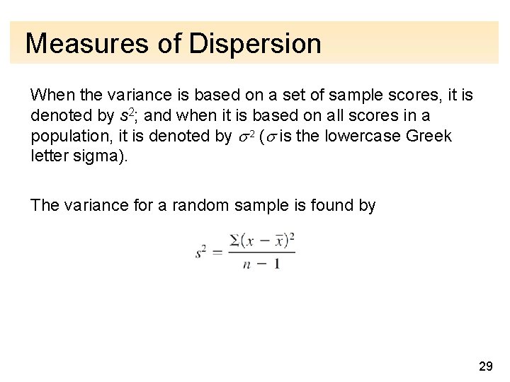
Measures of Dispersion When the variance is based on a set of sample scores, it is denoted by s 2; and when it is based on all scores in a population, it is denoted by 2 ( is the lowercase Greek letter sigma). The variance for a random sample is found by 29

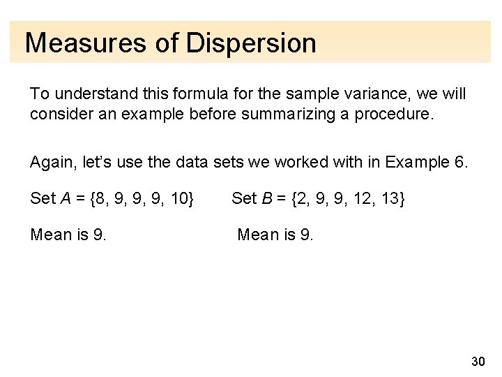
Measures of Dispersion To understand this formula for the sample variance, we will consider an example before summarizing a procedure. Again, let’s use the data sets we worked with in Example 6. Set A = {8, 9, 9, 9, 10} Mean is 9. Set B = {2, 9, 9, 12, 13} Mean is 9. 30

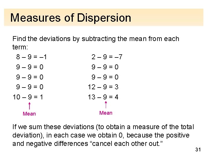
Measures of Dispersion Find the deviations by subtracting the mean from each term: 8 – 9 = – 1 2 – 9 = – 7 9– 9=0 9– 9=0 12 – 9 = 3 10 – 9 = 1 13 – 9 = 4 Mean If we sum these deviations (to obtain a measure of the total deviation), in each case we obtain 0, because the positive and negative differences “cancel each other out. ” 31

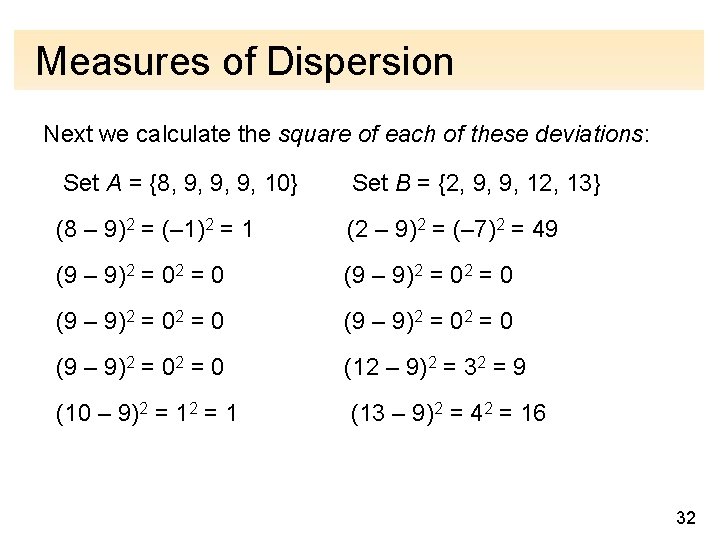
Measures of Dispersion Next we calculate the square of each of these deviations: Set A = {8, 9, 9, 9, 10} Set B = {2, 9, 9, 12, 13} (8 – 9)2 = (– 1)2 = 1 (2 – 9)2 = (– 7)2 = 49 (9 – 9)2 = 02 = 0 (9 – 9)2 = 0 (12 – 9)2 = 32 = 9 (10 – 9)2 = 1 (13 – 9)2 = 42 = 16 32

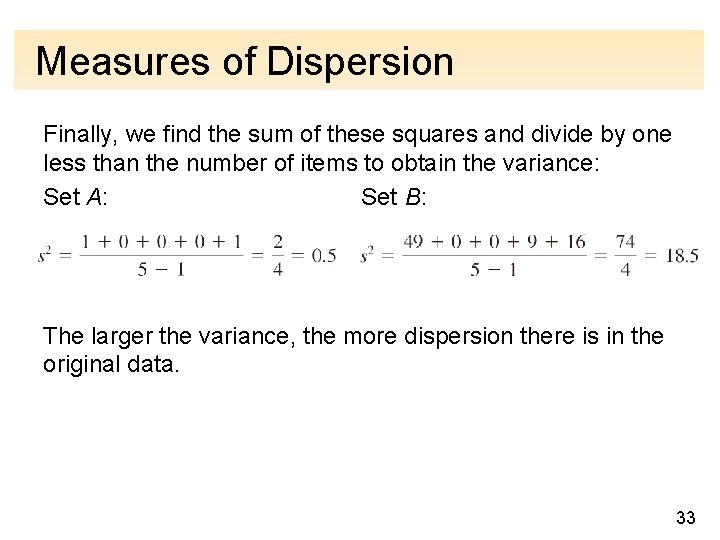
Measures of Dispersion Finally, we find the sum of these squares and divide by one less than the number of items to obtain the variance: Set A: Set B: The larger the variance, the more dispersion there is in the original data. 33

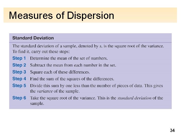
Measures of Dispersion 34

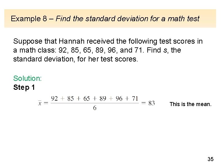
Example 8 – Find the standard deviation for a math test Suppose that Hannah received the following test scores in a math class: 92, 85, 65, 89, 96, and 71. Find s, the standard deviation, for her test scores. Solution: Step 1 This is the mean. 35

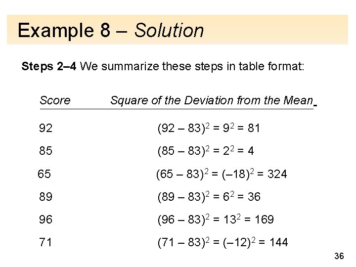
Example 8 – Solution Steps 2– 4 We summarize these steps in table format: Score Square of the Deviation from the Mean 92 (92 – 83)2 = 92 = 81 85 (85 – 83)2 = 22 = 4 65 (65 – 83) 2 = (– 18)2 = 324 89 (89 – 83)2 = 62 = 36 96 (96 – 83)2 = 132 = 169 71 (71 – 83)2 = (– 12)2 = 144 36

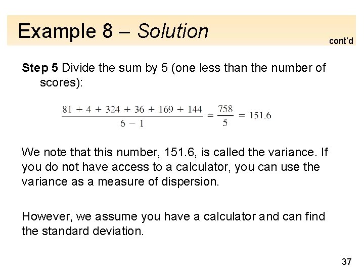
Example 8 – Solution cont’d Step 5 Divide the sum by 5 (one less than the number of scores): We note that this number, 151. 6, is called the variance. If you do not have access to a calculator, you can use the variance as a measure of dispersion. However, we assume you have a calculator and can find the standard deviation. 37

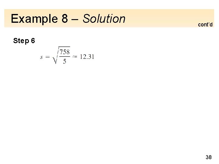
Example 8 – Solution cont’d Step 6 38

Interpreting Measures of Dispersion A main use of dispersion is to compare the amounts of spread in two (or more) data sets. A common technique in inferential statistics is to draw comparisons between populations by analyzing samples that come from those populations. 39 39

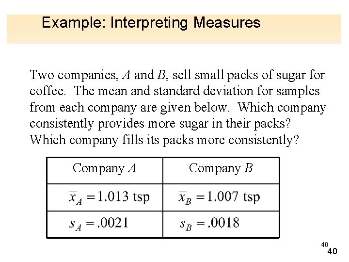
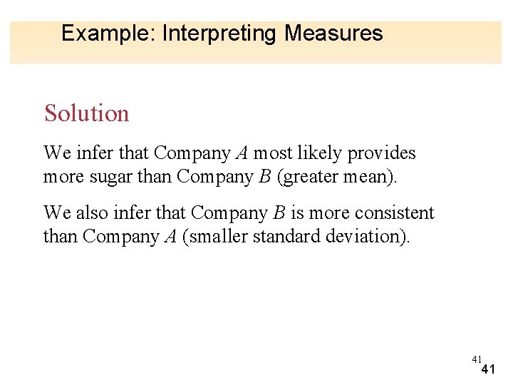
Example: Interpreting Measures Two companies, A and B, sell small packs of sugar for coffee. The mean and standard deviation for samples from each company are given below. Which company consistently provides more sugar in their packs? Which company fills its packs more consistently? Company A Company B 40 40

Example: Interpreting Measures Solution We infer that Company A most likely provides more sugar than Company B (greater mean). We also infer that Company B is more consistent than Company A (smaller standard deviation). 41 41

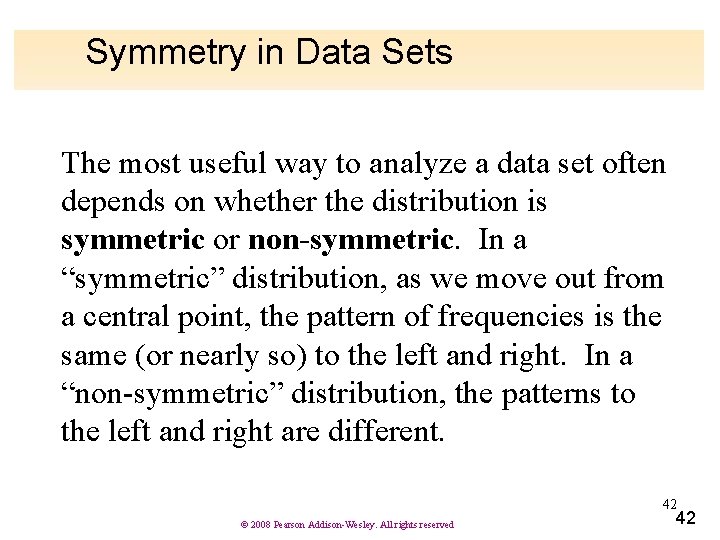
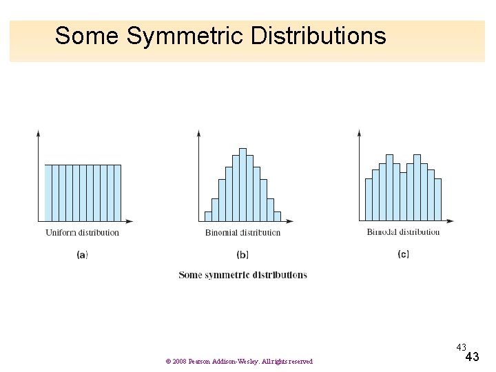
Symmetry in Data Sets The most useful way to analyze a data set often depends on whether the distribution is symmetric or non-symmetric. In a “symmetric” distribution, as we move out from a central point, the pattern of frequencies is the same (or nearly so) to the left and right. In a “non-symmetric” distribution, the patterns to the left and right are different. 42 © 2008 Pearson Addison-Wesley. All rights reserved 42

Some Symmetric Distributions 43 © 2008 Pearson Addison-Wesley. All rights reserved 43

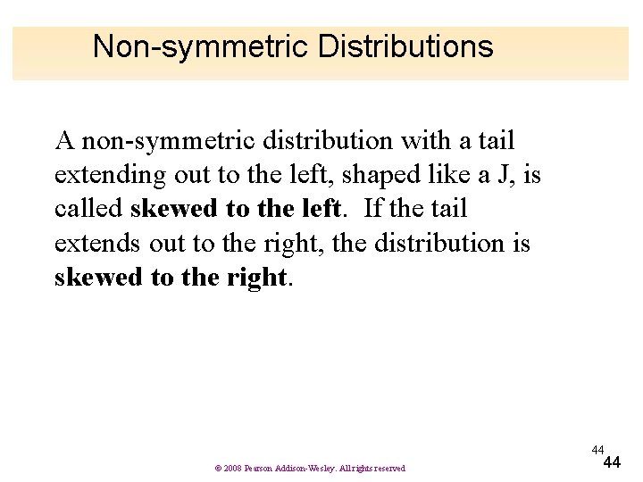
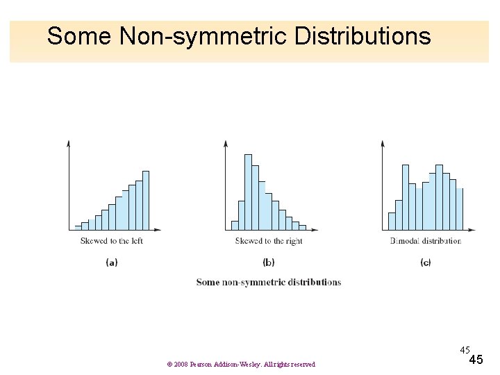
Non-symmetric Distributions A non-symmetric distribution with a tail extending out to the left, shaped like a J, is called skewed to the left. If the tail extends out to the right, the distribution is skewed to the right. 44 © 2008 Pearson Addison-Wesley. All rights reserved 44

Some Non-symmetric Distributions 45 © 2008 Pearson Addison-Wesley. All rights reserved 45

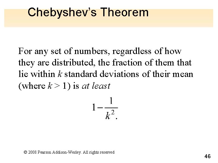
Chebyshev’s Theorem For any set of numbers, regardless of how they are distributed, the fraction of them that lie within k standard deviations of their mean (where k > 1) is at least © 2008 Pearson Addison-Wesley. All rights reserved 46

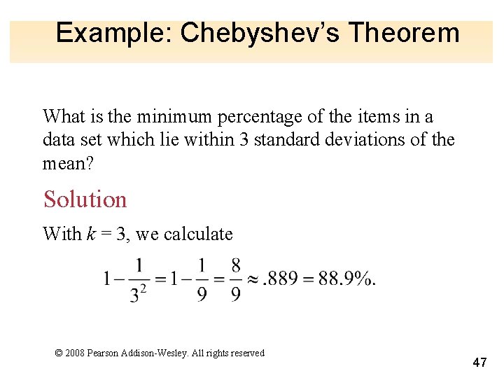
Example: Chebyshev’s Theorem What is the minimum percentage of the items in a data set which lie within 3 standard deviations of the mean? Solution With k = 3, we calculate © 2008 Pearson Addison-Wesley. All rights reserved 47