Intro to modeling April 22 2011 Part of

Intro to modeling April 22 2011

Part of the course: Introduction to biological modeling 1. Intro to modeling 2. Intro to biological modeling (Floor) 3. Modeling oscillators (Rob)

Today’s goal: Learn how to solve ODE models in MATLAB

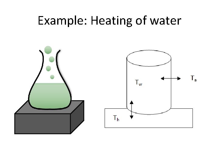
Example: Heating of water

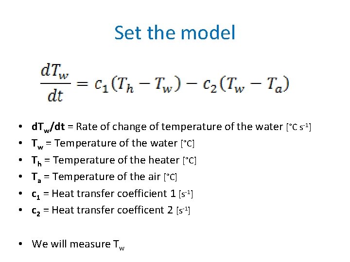
Set the model • • • d. Tw/dt = Rate of change of temperature of the water [°C s-1] Tw = Temperature of the water [°C] Th = Temperature of the heater [°C] Ta = Temperature of the air [°C] c 1 = Heat transfer coefficient 1 [s-1] c 2 = Heat transfer coefficent 2 [s-1] • We will measure Tw

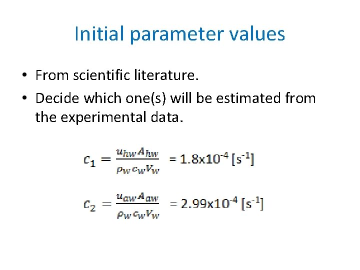
Initial parameter values • From scientific literature. • Decide which one(s) will be estimated from the experimental data.

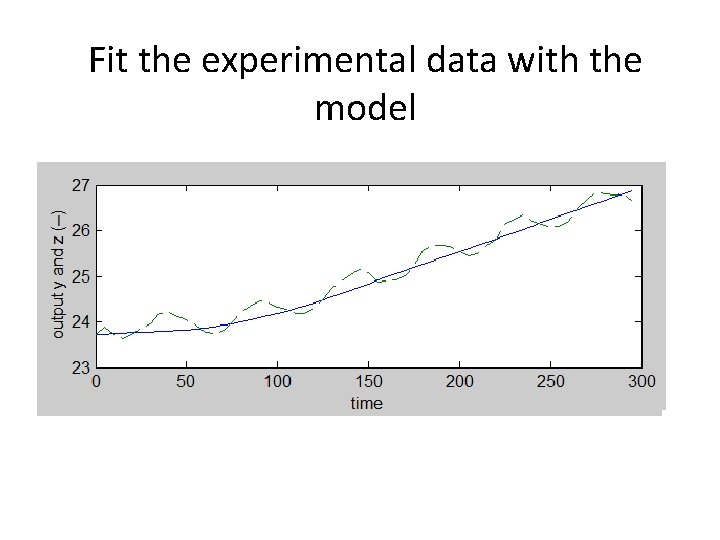
Fit the experimental data with the model

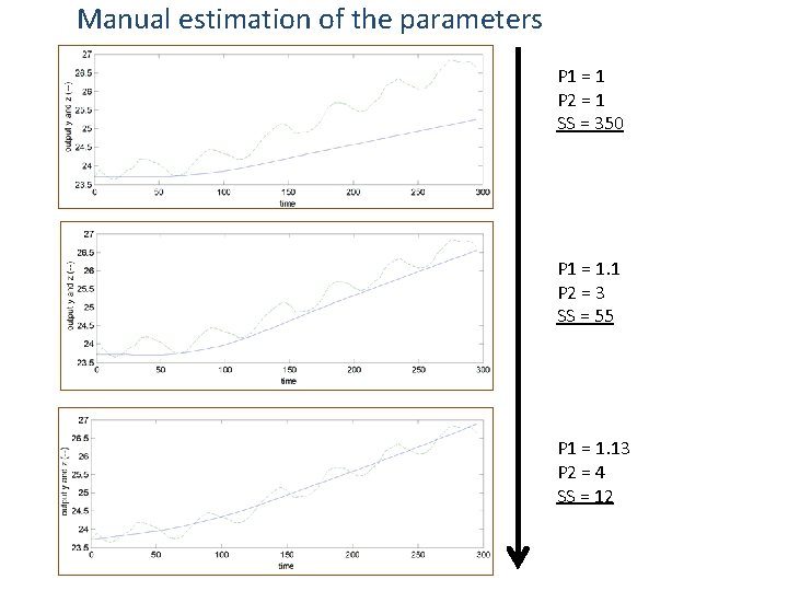
Manual estimation of the parameters P 1 = 1 P 2 = 1 SS = 350 P 1 = 1. 1 P 2 = 3 SS = 55 P 1 = 1. 13 P 2 = 4 SS = 12

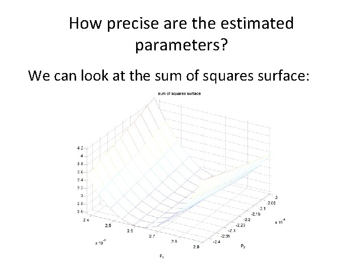
How precise are the estimated parameters? We can look at the sum of squares surface:

Why modeling? • Simulate the system • Estimate parameters • Control the system

Menu § The math behind modeling (45 min) § Break (5 min) § A few words about programming (10 min) § Hands-on tutorial (45 min) § What’s next (5 min)

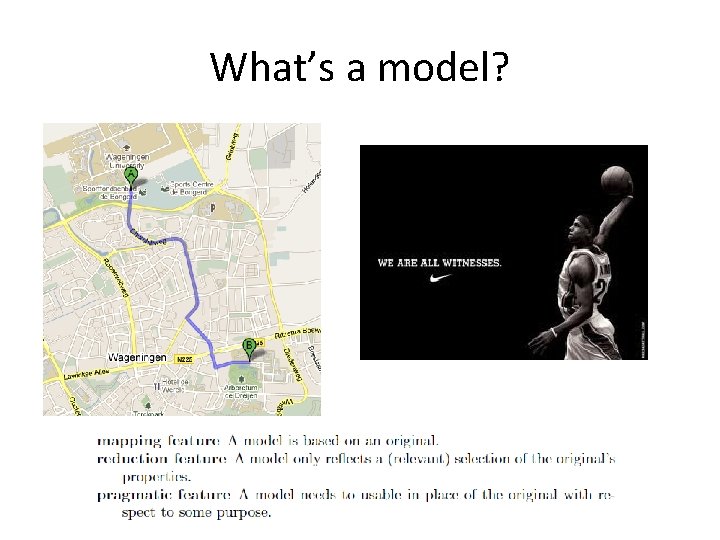
What’s a model?

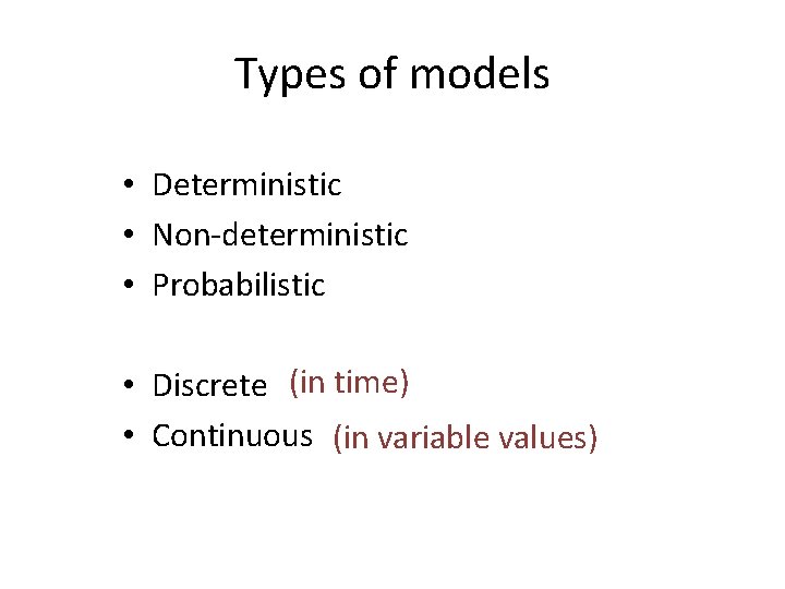
Types of models • Deterministic • Non-deterministic • Probabilistic • Discrete (in time) • Continuous (in variable values)

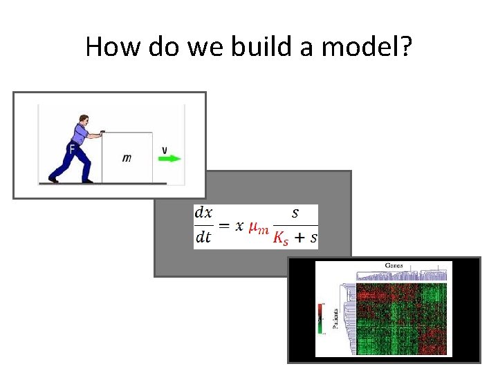
How do we build a model? White box: First principles Grey box Black box: Measurements

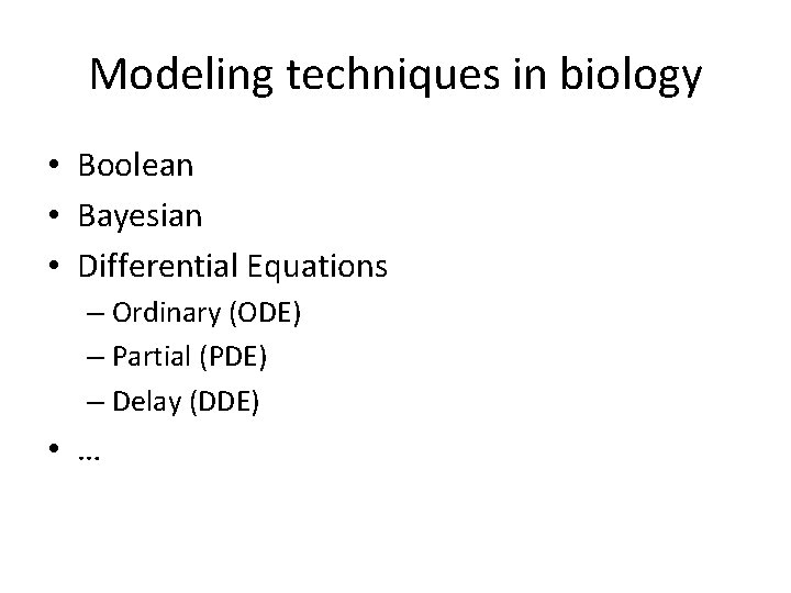
Modeling techniques in biology • Boolean • Bayesian • Differential Equations – Ordinary (ODE) – Partial (PDE) – Delay (DDE) • …

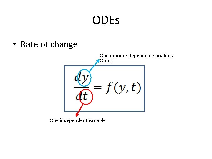
ODEs • Rate of change One or more dependent variables Order One independent variable

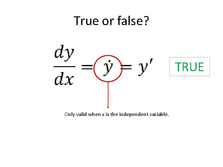
True or false? TRUE Only valid when x is the independent variable.

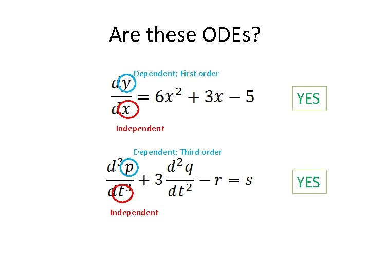
Are these ODEs? Dependent; First order YES Independent Dependent; Third order YES Independent

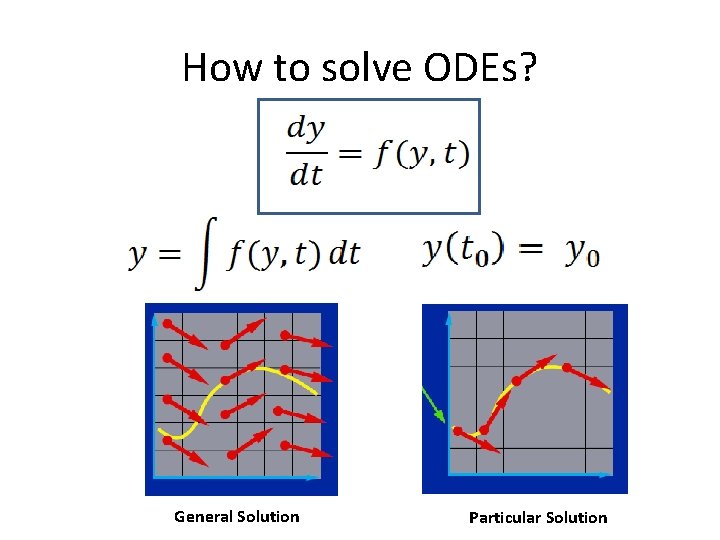
How to solve ODEs? General Solution Particular Solution

How to solve ODEs? • Analytical or • Numerical solution – Euler – ode 45

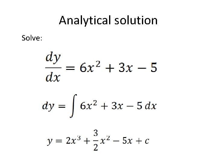
Analytical solution Solve:

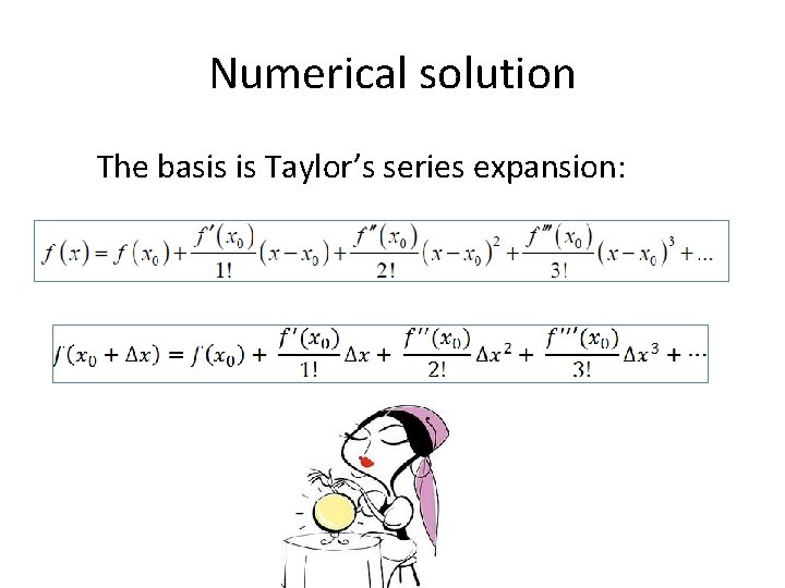
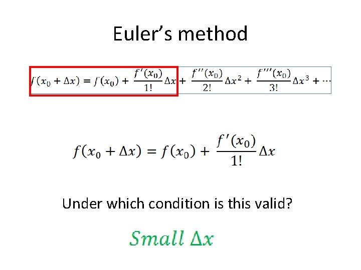
Numerical solution The basis is Taylor’s series expansion:

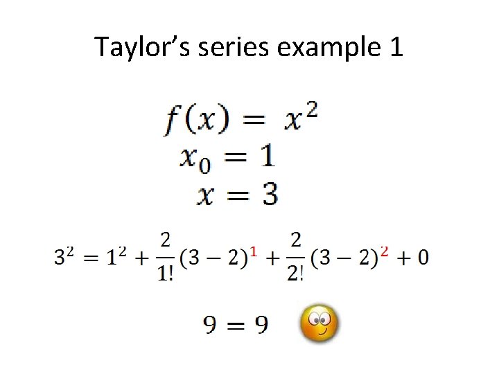
Taylor’s series example 1

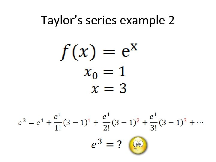
Taylor’s series example 2

Euler’s method Under which condition is this valid?

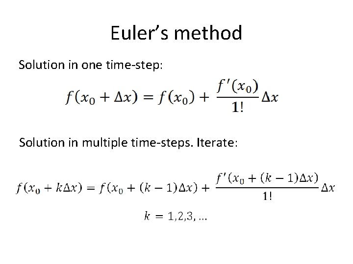
Euler’s method Solution in one time-step: Solution in multiple time-steps. Iterate:

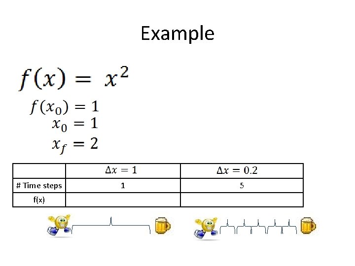
Example # Time steps f(x) 1 5

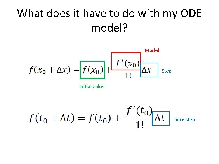
What does it have to do with my ODE model? Model Step Initial value Time step

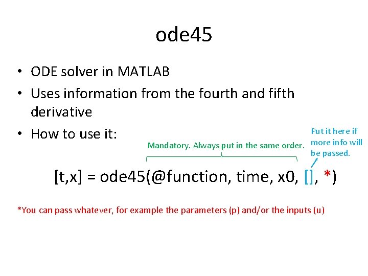
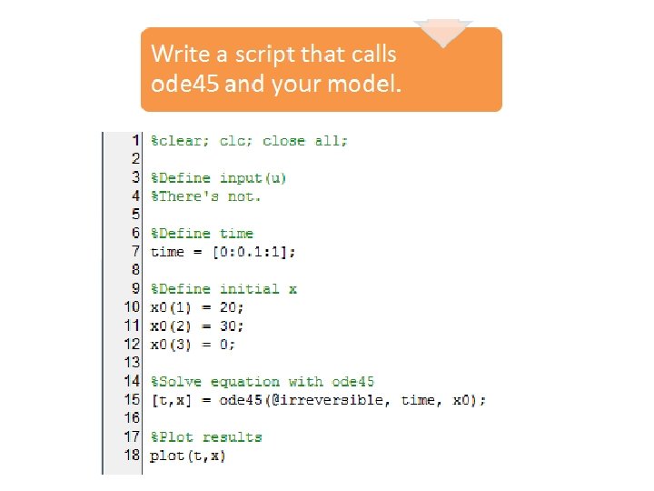
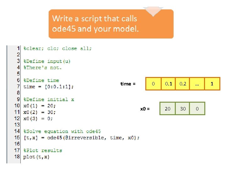
ode 45 • ODE solver in MATLAB • Uses information from the fourth and fifth derivative • How to use it: Put it here if Mandatory. Always put in the same order. more info will be passed. [t, x] = ode 45(@function, time, x 0, [], *) *You can pass whatever, for example the parameters (p) and/or the inputs (u)

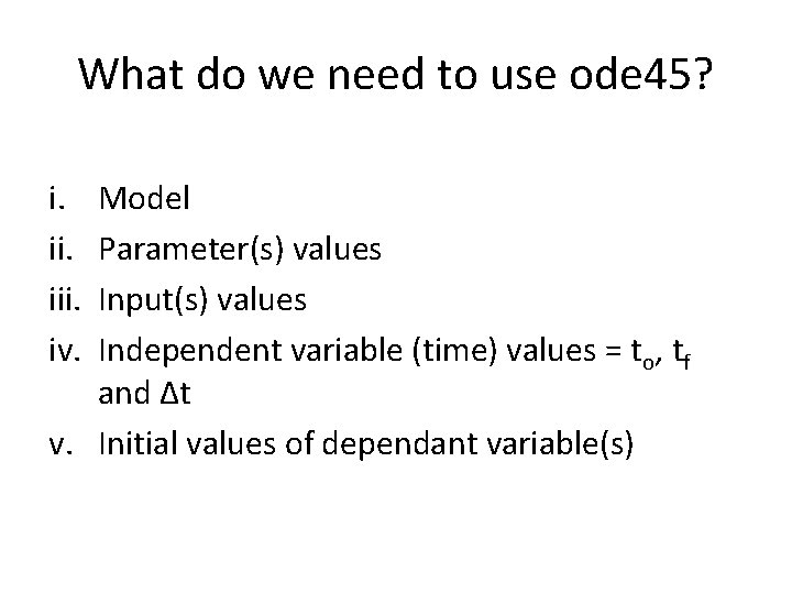
What do we need to use ode 45? i. iii. iv. Model Parameter(s) values Input(s) values Independent variable (time) values = to, tf and Δt v. Initial values of dependant variable(s)

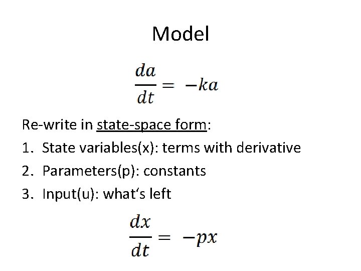
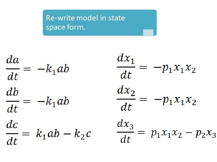
Model Re-write in state-space form: 1. State variables(x): terms with derivative 2. Parameters(p): constants 3. Input(u): what‘s left

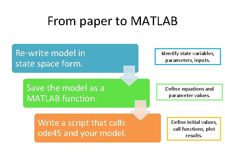
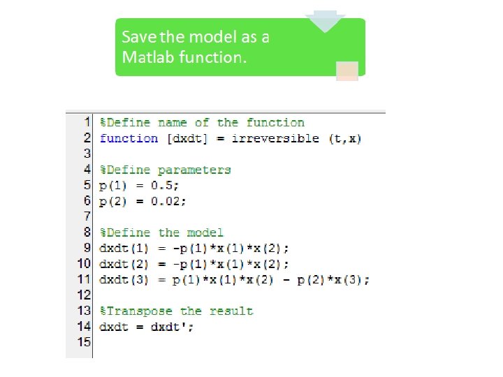
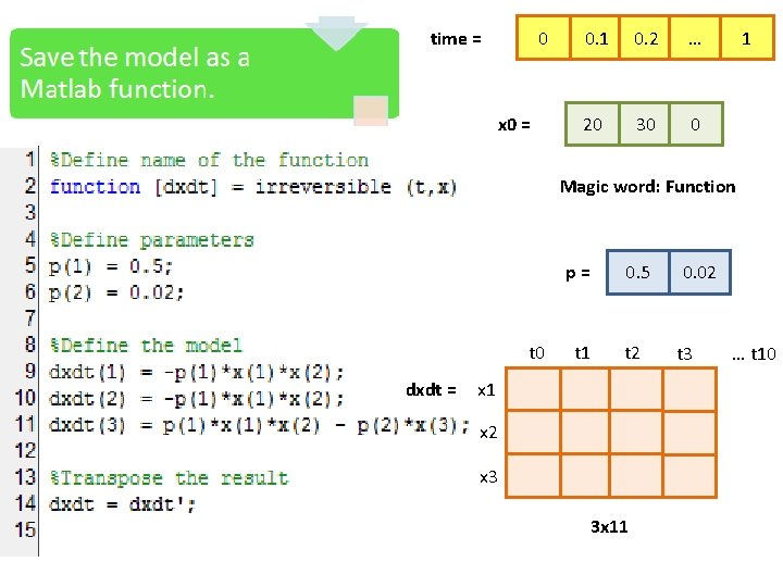
From paper to MATLAB Re-write model in state space form. Save the model as a MATLAB function. Write a script that calls ode 45 and your model. Identify state variables, parameters, inputs. Define equations and parameter values. Define initial values, call functions, plot results.

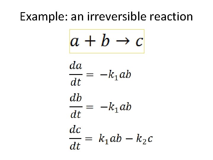
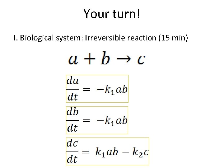
Example: an irreversible reaction

Now the language details…

0 time = x 0 = 0. 1 0. 2 … 20 30 0 1

0 time = x 0 = 0. 1 0. 2 … 20 30 0 1 Magic word: Function p= t 0 dxdt = t 1 0. 5 0. 02 t 3 x 1 x 2 x 3 3 x 11 … t 10

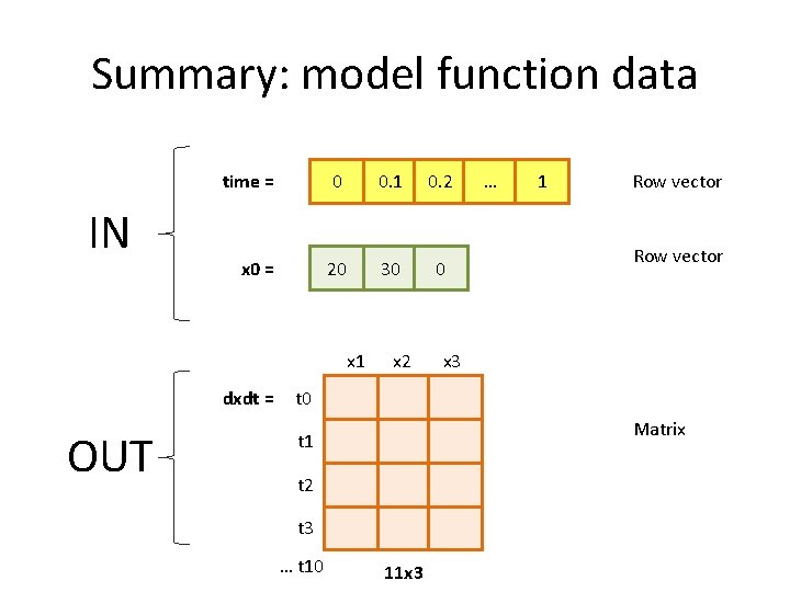
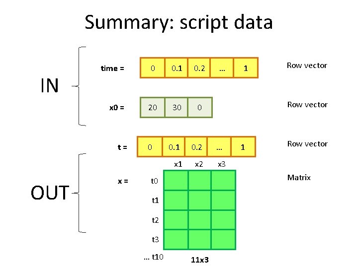
Summary: model function data IN time = 0 0. 1 0. 2 x 0 = 20 30 0 x 1 dxdt = OUT x 2 … 1 Row vector x 3 t 0 Matrix t 1 t 2 t 3 … t 10 11 x 3

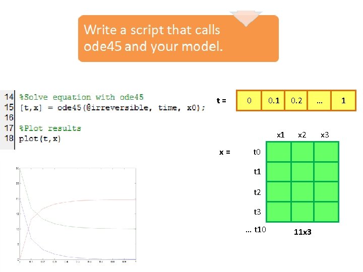
t= 0 0. 1 x= 0. 2 x 2 t 0 t 1 t 2 t 3 … t 10 11 x 3 … x 3 1

Summary: script data IN time = 0 0. 1 0. 2 x 0 = 20 30 0 0. 1 0. 2 … x 1 x 2 x 3 t= OUT x= 0 1 Row vector Matrix t 0 t 1 t 2 t 3 … t 10 … 11 x 3

From paper to MATLAB Re-write model in state space form. Save the model as a MATLAB function. Write a script that calls ode 45 and your model. Identify state variables, parameters, inputs. Define equations and parameter values. Define initial values, call functions, plot results.

Break

A few words about programming Ø All programs run in a defined ‘vertical’ way. Ø MATLAB is an interpreted language. ØErrors can be found at any time. Ø Read the errors messages. ØMost errors are in manipulation of row/column vectors.

A few words about programming • Shell/command line = type commands interactively • Scripts (. m) = save commands • Functions (. m) = define a command. Give same name to the function and the file. • Variables – Any word/letter that stores data – They remain after the program ends • Semicolon (; )

Hands-on Tutorial

Your turn! I. Biological system: Irreversible reaction (15 min)

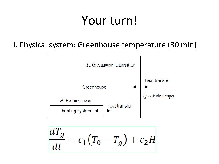
Your turn! I. Physical system: Greenhouse temperature (30 min)

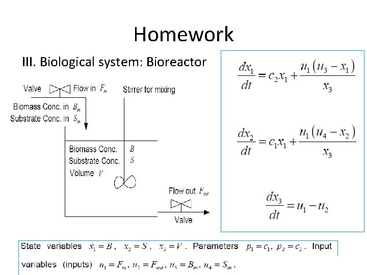
Homework III. Biological system: Bioreactor

What’s next Learn/Teach: q Introduction to biological modeling (Floor) q Modeling oscillators (Rob) Reproduce modeling by Danino et al. 2010: q MATLAB 7. 0 q Team: Brendan, Floor, Rob, Dorett, Mariana, . . . May 6 th presentation