Intro to Data Mining for Data Science Peter

Intro to Data Mining for Data Science Peter Fox Data Science – ITEC/CSCI/ERTH-4750/6750 Week 9, October 21, 2014 1

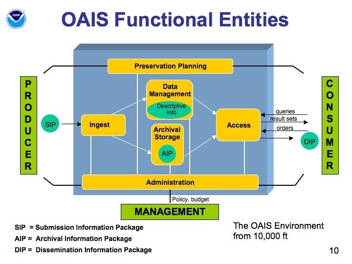
2

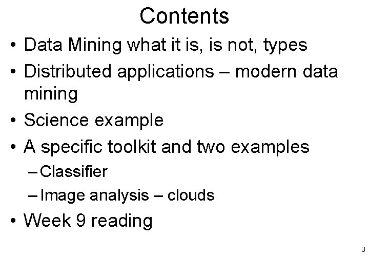
Contents • Data Mining what it is, is not, types • Distributed applications – modern data mining • Science example • A specific toolkit and two examples – Classifier – Image analysis – clouds • Week 9 reading 3

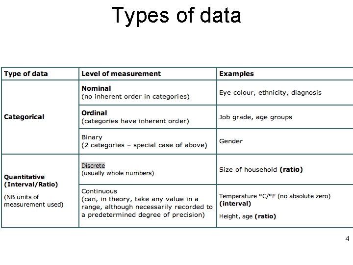
Types of data 4

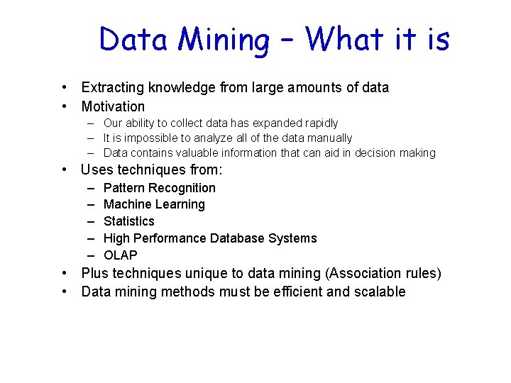
Data Mining – What it is • Extracting knowledge from large amounts of data • Motivation – Our ability to collect data has expanded rapidly – It is impossible to analyze all of the data manually – Data contains valuable information that can aid in decision making • Uses techniques from: – – – Pattern Recognition Machine Learning Statistics High Performance Database Systems OLAP • Plus techniques unique to data mining (Association rules) • Data mining methods must be efficient and scalable

Data Mining – What it isn’t • Small Scale – Data mining methods are designed for large data sets – Scale is one of the characteristics that distinguishes data mining applications from traditional machine learning applications • Foolproof – – Data mining techniques will discover patterns in any data The patterns discovered may be meaningless It is up to the user to determine how to interpret the results “Make it foolproof and they’ll just invent a better fool” • Magic – Data mining techniques cannot generate information that is not present in the data – They can only find the patterns that are already there

Data Mining – Types of Mining • Classification (Supervised Learning) – Classifiers are created using labeled training samples – Training samples created by ground truth / experts – Classifier later used to classify unknown samples • Clustering (Unsupervised Learning) – Grouping objects into classes so that similar objects are in the same class and dissimilar objects are in different classes – Discoverall distribution patterns and relationships between attributes • Association Rule Mining – Initially developed for market basket analysis – Goal is to discover relationships between attributes – Uses include decision support, classification and clustering • Other Types of Mining – Outlier Analysis – Concept / Class Description – Time Series Analysis

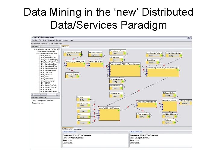
Data Mining in the ‘new’ Distributed Data/Services Paradigm

Science Motivation • Study the impact of natural iron fertilization process (such as a dust storm) on plankton growth and subsequent dimethyl sulfide (DMS) production – Plankton plays an important role in the carbon cycle – Plankton growth is strongly influenced by nutrient availability (Fe/Ph) – Dust deposition is important source of Fe over ocean – Satellite data is an effective tool for monitoring the effects of dust fertilization

Hypotheses • In remote ocean locations there is a positive correlation between the area averaged atmospheric aerosol loading and oceanic chlorophyll concentration • There is a time lag between oceanic dust deposition and the photosynthetic activity

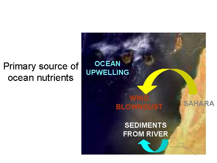
Primary source of ocean nutrients OCEAN UPWELLING WIND BLOWNDUST SEDIMENTS FROM RIVER SAHARA

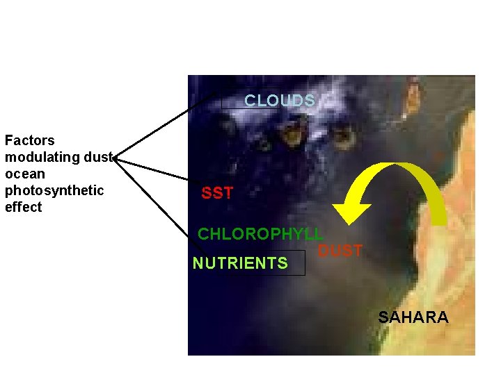
CLOUDS Factors modulating dustocean photosynthetic effect SST CHLOROPHYLL DUST NUTRIENTS SAHARA

Objectives • Use satellite data to determine, if atmospheric dust loading and phytoplankton photosynthetic activity are correlated. • Determine physical processes responsible for observed relationship

Data and Method • Data sets obtained from two instruments: Sea. Wi. FS and MODIS during 2000 – 2006 are employed • MODIS derived AOT (Aerosol Optical Thickness) – Sea. WIFS - Sea-Viewing Wide Field-of-View Sensor – MODIS – Moderate resolution Imaging Spectrometer – AOT – Aerosol Optical Thickness

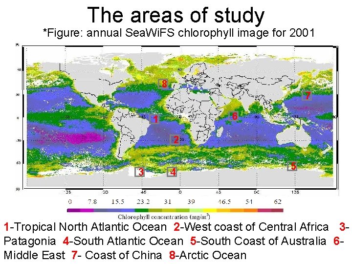
The areas of study *Figure: annual Sea. Wi. FS chlorophyll image for 2001 8 7 6 1 2 3 4 5 1 -Tropical North Atlantic Ocean 2 -West coast of Central Africa 3 Patagonia 4 -South Atlantic Ocean 5 -South Coast of Australia 6 Middle East 7 - Coast of China 8 -Arctic Ocean

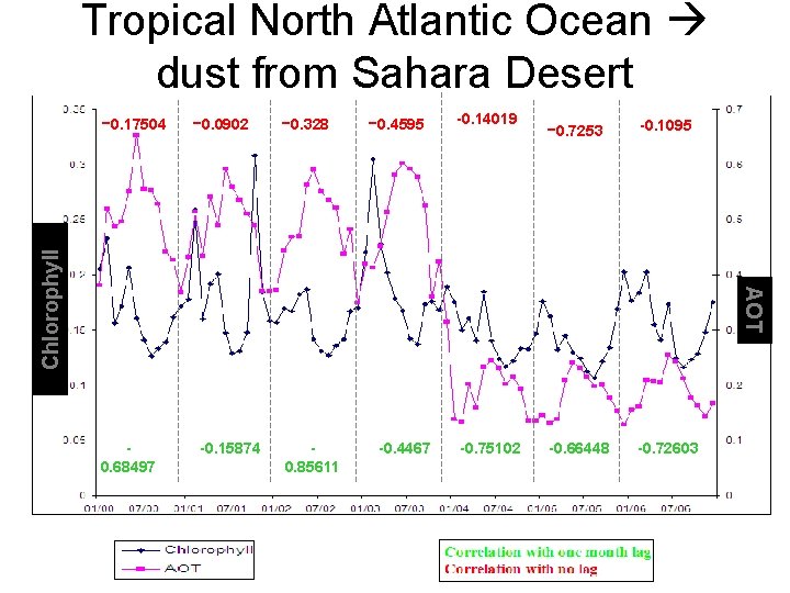
Tropical North Atlantic Ocean dust from Sahara Desert -0. 0902 -0. 328 -0. 4595 -0. 14019 -0. 7253 -0. 1095 -0. 75102 -0. 66448 -0. 72603 AOT Chlorophyll -0. 17504 0. 68497 -0. 15874 0. 85611 -0. 4467

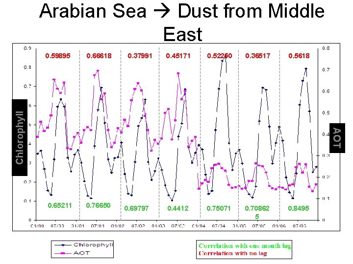
Arabian Sea Dust from Middle East 0. 66618 0. 37991 0. 45171 0. 52250 0. 36517 0. 5618 0. 4412 0. 75071 0. 70862 5 0. 8495 AOT Chlorophyll 0. 59895 0. 65211 0. 76650 0. 69797

Summary … • Dust impacts oceans photosynthetic activity, positive correlations in some areas NEGATIVE correlation in other areas, especially in the Saharan basin • Hypothesis for explaining observations of negative correlation: In areas that are not nutrient limited, dust reduces photosynthetic activity • But also need to consider the effect of clouds, ocean currents. Also need to isolate the effects of dust. MODIS AOT product includes contribution from dust, DMS, biomass burning etc.

Data Mining – Types of Mining • Classification (Supervised Learning) – Classifiers are created using labeled training samples – Training samples created by ground truth / experts – Classifier later used to classify unknown samples • Clustering (Unsupervised Learning) – Grouping objects into classes so that similar objects are in the same class and dissimilar objects are in different classes – Discoverall distribution patterns and relationships between attributes • Association Rule Mining – Initially developed for market basket analysis – Goal is to discover relationships between attributes – Uses include decision support, classification and clustering • Other Types of Mining – Outlier Analysis – Concept / Class Description – Time Series Analysis

Models/ types • Trade-off between Accuracy and Understandability • Models range from “easy to understand” to incomprehensible – Decision trees – Rule induction – Regression models – Neural Networks H a r d e r 20

Qualitative and Quantitative • Qualitative – Provide insight into the data you are working with • If city = New York and 30 < age < 35 … • Important age demographic was previously 20 to 25 • Change print campaign from Village Voice to New Yorker – Requires interaction capabilities and good visualization • Quantitative • Automated process • Score new gene chip datasets with error model every night at midnight • Bottom-line orientation 21

Management • • • Creation of logical collections Physical data handling Interoperability support Security support Data ownership Metadata collection, management and access. Persistence Knowledge and information discovery Data dissemination and publication 22

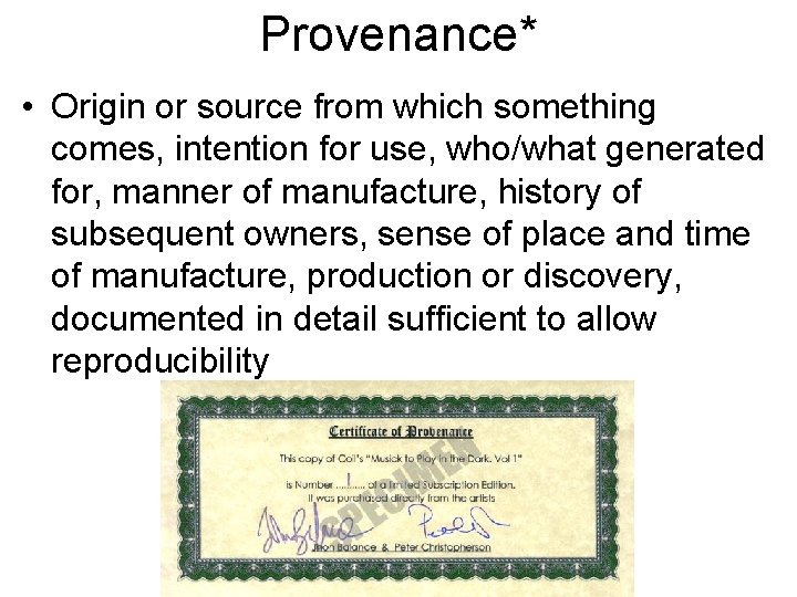
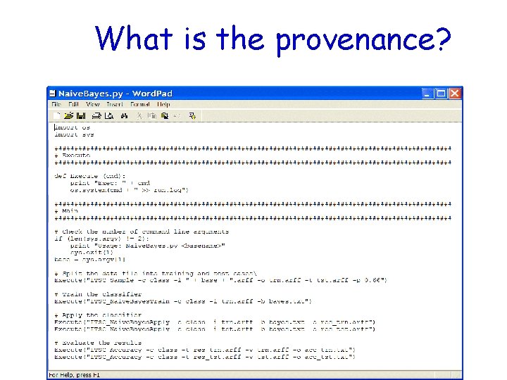
Provenance* • Origin or source from which something comes, intention for use, who/what generated for, manner of manufacture, history of subsequent owners, sense of place and time of manufacture, production or discovery, documented in detail sufficient to allow reproducibility

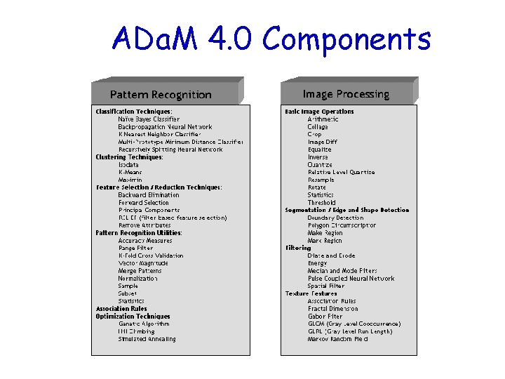
ADa. M – System Overview • Developed by the Information Technology and Systems Center at the University of Alabama in Huntsville • Consists of over 75 interoperable mining and image processing components • Each component is provided with a C++ application programming interface (API), an executable in support of scripting tools (e. g. Perl, Python, Tcl, Shell) • ADa. M components are lightweight and autonomous, and have been used successfully in a grid environment • ADa. M has several translation components that provide data level interoperability with other mining systems (such as WEKA and Orange), and point tools (such as lib. SVM and svm. Light) • Future versions will include Python wrappers and possible web service interfaces

ADa. M 4. 0 Components

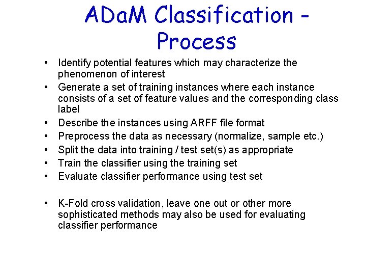
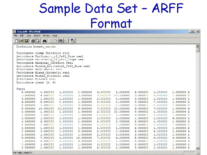
ADa. M Classification Process • Identify potential features which may characterize the phenomenon of interest • Generate a set of training instances where each instance consists of a set of feature values and the corresponding class label • Describe the instances using ARFF file format • Preprocess the data as necessary (normalize, sample etc. ) • Split the data into training / test set(s) as appropriate • Train the classifier using the training set • Evaluate classifier performance using test set • K-Fold cross validation, leave one out or other more sophisticated methods may also be used for evaluating classifier performance

ADa. M Classification Example • Starting with an ARFF file, the ADa. M system will be used to create a Naïve Bayes classifier and evaluate it • The source data will be an ARFF version of the Wisconsin breast cancer data from the University of California Irvine (UCI) Machine Learning Database: http: //www. ics. uci. edu/~mlearn/MLRepository. html • The Naïve Bayes classifier will be trained to distinguish malignant vs. benign tumors based on nine characteristics

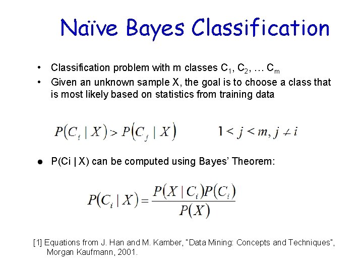
Naïve Bayes Classification • Classification problem with m classes C 1, C 2, … Cm • Given an unknown sample X, the goal is to choose a class that is most likely based on statistics from training data l P(Ci | X) can be computed using Bayes’ Theorem: [1] Equations from J. Han and M. Kamber, “Data Mining: Concepts and Techniques”, Morgan Kaufmann, 2001.

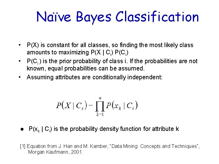
Naïve Bayes Classification • P(X) is constant for all classes, so finding the most likely class amounts to maximizing P(X | Ci) P(Ci) • P(Ci ) is the prior probability of class i. If the probabilities are not known, equal probabilities can be assumed. • Assuming attributes are conditionally independent: l P(xk | Ci) is the probability density function for attribute k [1] Equation from J. Han and M. Kamber, “Data Mining: Concepts and Techniques”, Morgan Kaufmann, 2001.

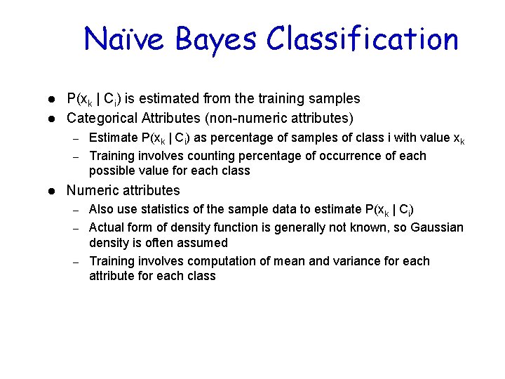
Naïve Bayes Classification l l P(xk | Ci) is estimated from the training samples Categorical Attributes (non-numeric attributes) – – l Estimate P(xk | Ci) as percentage of samples of class i with value xk Training involves counting percentage of occurrence of each possible value for each class Numeric attributes – – – Also use statistics of the sample data to estimate P(xk | Ci) Actual form of density function is generally not known, so Gaussian density is often assumed Training involves computation of mean and variance for each attribute for each class

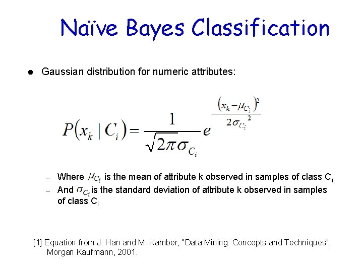
Naïve Bayes Classification l Gaussian distribution for numeric attributes: – – Where is the mean of attribute k observed in samples of class Ci And is the standard deviation of attribute k observed in samples of class Ci [1] Equation from J. Han and M. Kamber, “Data Mining: Concepts and Techniques”, Morgan Kaufmann, 2001.

Sample Data Set – ARFF Format

Data management • • Metadata? Data? File naming? Documentation?

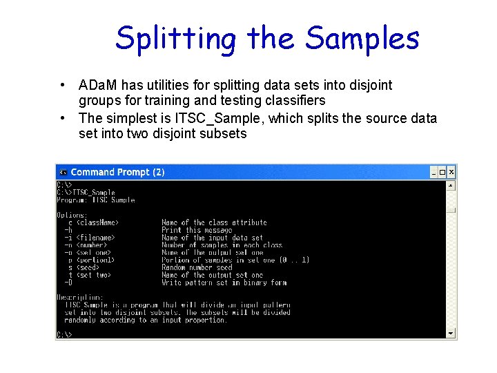
Splitting the Samples • ADa. M has utilities for splitting data sets into disjoint groups for training and testing classifiers • The simplest is ITSC_Sample, which splits the source data set into two disjoint subsets

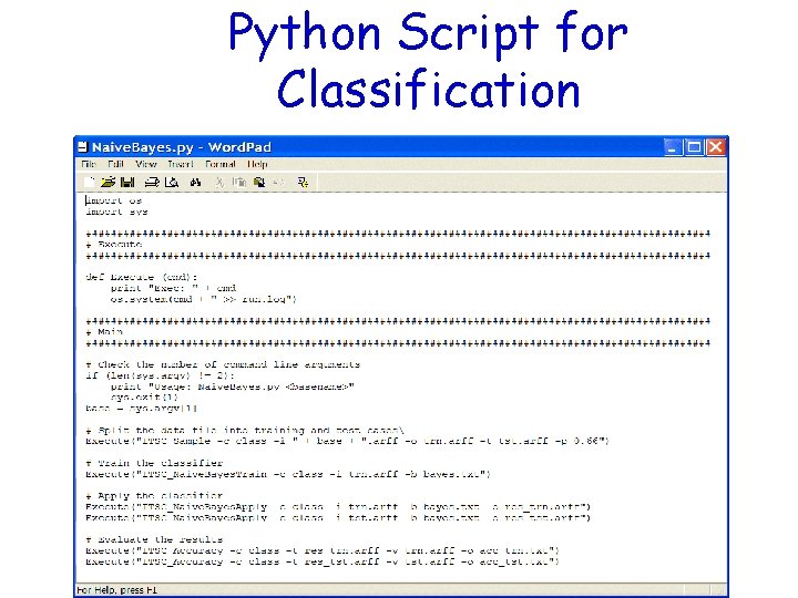
Splitting the Samples • For this demo, we will split the breast cancer data set into two groups, one with 2/3 of the patterns and another with 1/3 of the patterns: ITSC_Sample -c class -i bcw. arff -o trn. arff -t tst. arff –p 0. 66 • The –i argument specifies the input file name • The –o and –t arguments specify the names of the two output files (-o = output one, -t = output two) • The –p argument specifies the portion of data that goes into output one (trn. arff), the remainder goes to output two (tst. arff) • The –c argument tells the sample program which attribute is the class attribute

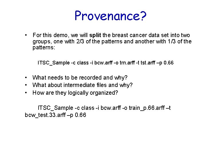
Provenance? • For this demo, we will split the breast cancer data set into two groups, one with 2/3 of the patterns and another with 1/3 of the patterns: ITSC_Sample -c class -i bcw. arff -o trn. arff -t tst. arff –p 0. 66 • What needs to be recorded and why? • What about intermediate files and why? • How are they logically organized? ITSC_Sample -c class -i bcw. arff -o train_p. 66. arff –t bcw_test. 33. arff –p 0. 66

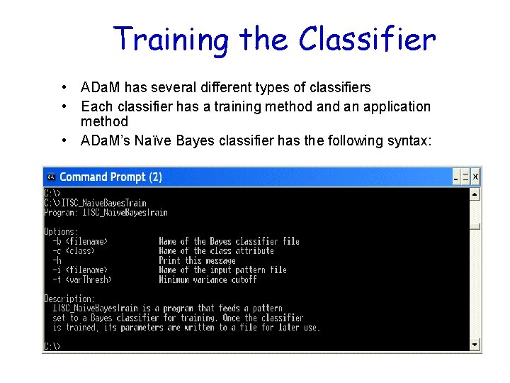
Training the Classifier • ADa. M has several different types of classifiers • Each classifier has a training method an application method • ADa. M’s Naïve Bayes classifier has the following syntax:

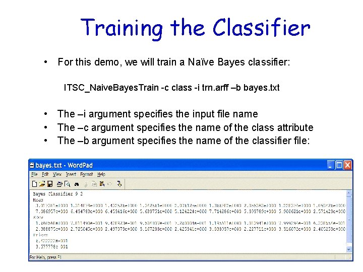
Training the Classifier • For this demo, we will train a Naïve Bayes classifier: ITSC_Naive. Bayes. Train -c class -i trn. arff –b bayes. txt • The –i argument specifies the input file name • The –c argument specifies the name of the class attribute • The –b argument specifies the name of the classifier file:

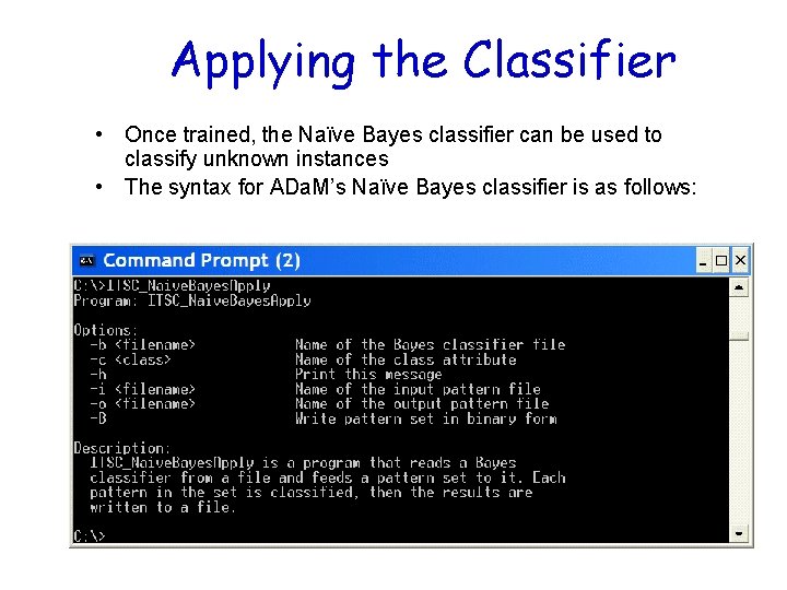
Applying the Classifier • Once trained, the Naïve Bayes classifier can be used to classify unknown instances • The syntax for ADa. M’s Naïve Bayes classifier is as follows:

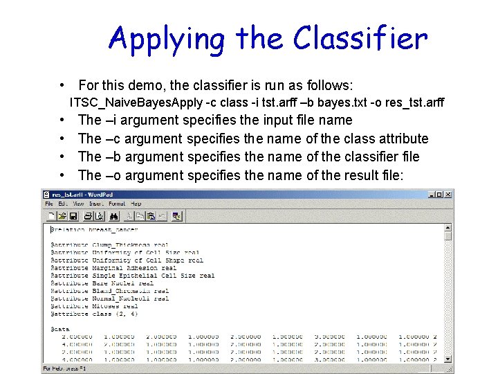
Applying the Classifier • For this demo, the classifier is run as follows: ITSC_Naive. Bayes. Apply -c class -i tst. arff –b bayes. txt -o res_tst. arff • • The –i argument specifies the input file name The –c argument specifies the name of the class attribute The –b argument specifies the name of the classifier file The –o argument specifies the name of the result file:

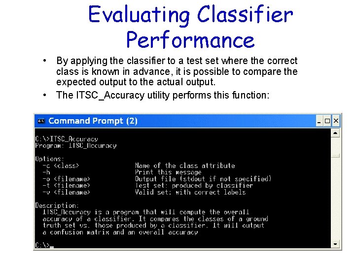
Evaluating Classifier Performance • By applying the classifier to a test set where the correct class is known in advance, it is possible to compare the expected output to the actual output. • The ITSC_Accuracy utility performs this function:

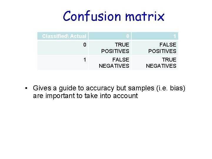
Confusion matrix Classified Actual 0 1 0 TRUE POSITIVES FALSE POSITIVES 1 FALSE NEGATIVES TRUE NEGATIVES • Gives a guide to accuracy but samples (i. e. bias) are important to take into account

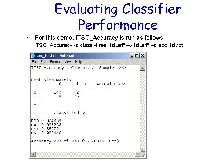
Evaluating Classifier Performance • For this demo, ITSC_Accuracy is run as follows: ITSC_Accuracy -c class -t res_tst. arff –v tst. arff –o acc_tst. txt

Python Script for Classification

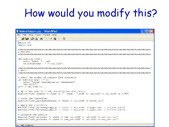
How would you modify this?

What is the provenance?

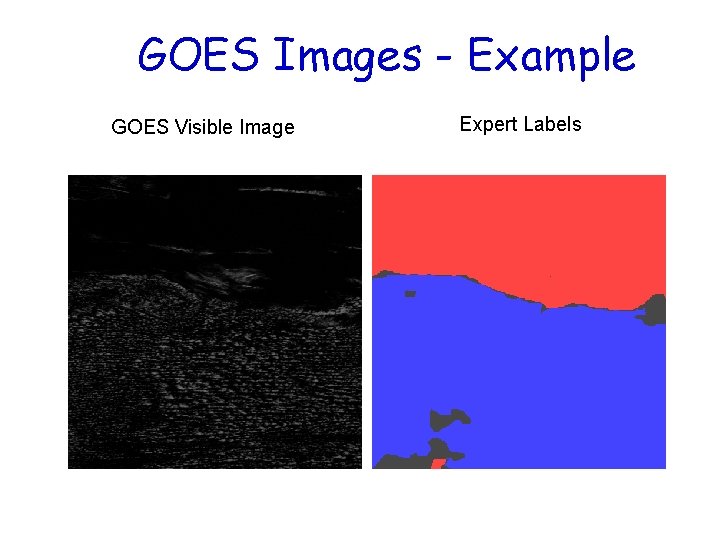
ADa. M Image Classification • Classification of image data is a bit more involved, as there is an additional set of steps that must be performed to extract useful features from the images before classification can be performed. • In addition, it is also useful to transform the data back into image format for visualization purposes. • As an example problem, we will consider detection of cumulus cloud fields in GOES satellite images – GOES satellites produce a 5 channel image every 15 minutes – The classifier must label each pixel as either belonging to a cumulus cloud field or not based on the GOES data – Algorithms based on spectral properties often miss cumulus clouds because of the low resolution of the IR channels and the small size of clouds – Texture features computed from the GOES visible image provide a means to detect cumulus cloud fields.

GOES Images Preprocessing • Segmentation is based only on the high resolution (1 km) visible channel. • In order to remove the effects of the light reflected from the Earth’s surface, a visible reference background image is constructed for each time of the day. • The reference image is subtracted from the visible image before it is segmented. • GOES image patches containing cumulus cloud regions, other cloud regions, and background were selected • Independent experts labeled each pixel of the selected image patches as cumulus cloud or not • The expert labels were combined to form a single “truth” image for each of the original image patches. In cases where the experts disagreed, the truth image was given a “don’t know” value

GOES Images - Example GOES Visible Image Expert Labels

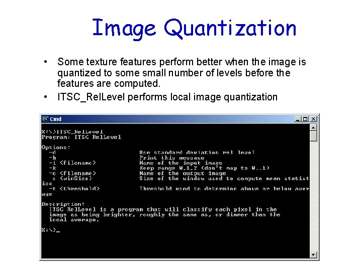
Image Quantization • Some texture features perform better when the image is quantized to some small number of levels before the features are computed. • ITSC_Rel. Level performs local image quantization

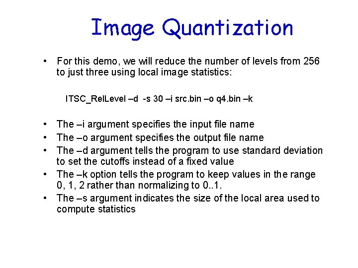
Image Quantization • For this demo, we will reduce the number of levels from 256 to just three using local image statistics: ITSC_Rel. Level –d -s 30 –i src. bin –o q 4. bin –k • The –i argument specifies the input file name • The –o argument specifies the output file name • The –d argument tells the program to use standard deviation to set the cutoffs instead of a fixed value • The –k option tells the program to keep values in the range 0, 1, 2 rather than normalizing to 0. . 1. • The –s argument indicates the size of the local area used to compute statistics

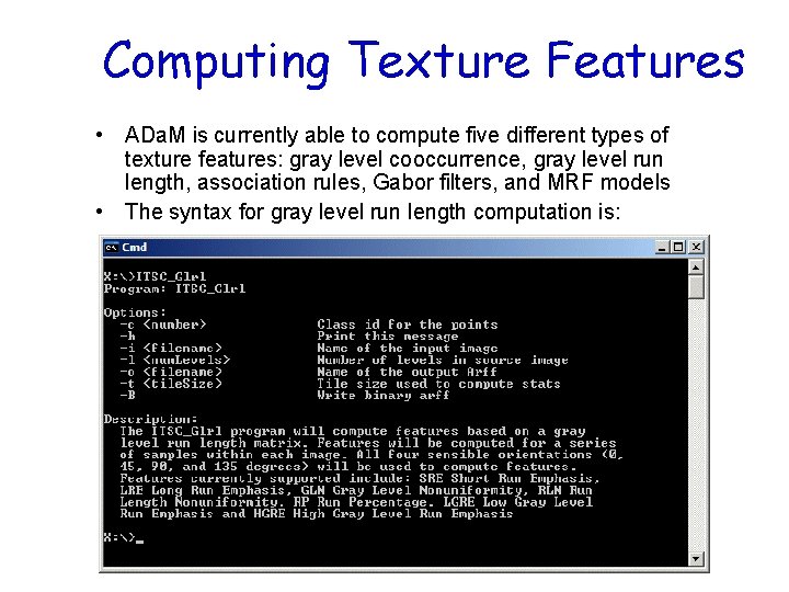
Computing Texture Features • ADa. M is currently able to compute five different types of texture features: gray level cooccurrence, gray level run length, association rules, Gabor filters, and MRF models • The syntax for gray level run length computation is:

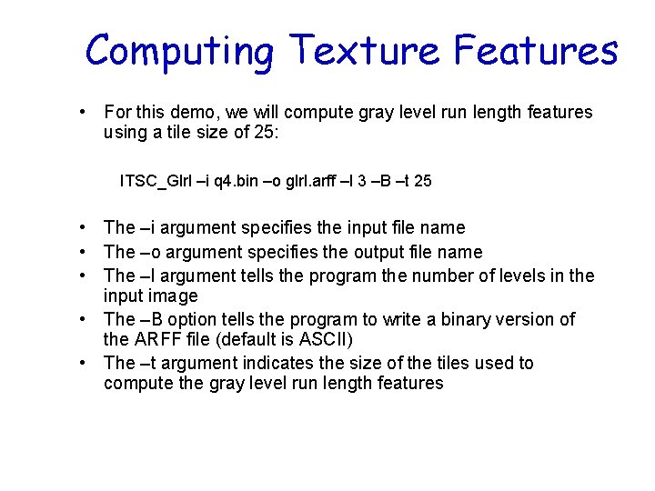
Computing Texture Features • For this demo, we will compute gray level run length features using a tile size of 25: ITSC_Glrl –i q 4. bin –o glrl. arff –l 3 –B –t 25 • The –i argument specifies the input file name • The –o argument specifies the output file name • The –l argument tells the program the number of levels in the input image • The –B option tells the program to write a binary version of the ARFF file (default is ASCII) • The –t argument indicates the size of the tiles used to compute the gray level run length features

Provenance alert! • For this demo, we will compute gray level run length features using a tile size of 25: ITSC_Glrl –i q 4. bin –o glrl. arff –l 3 –B –t 25 • What needs to be documented here and why?

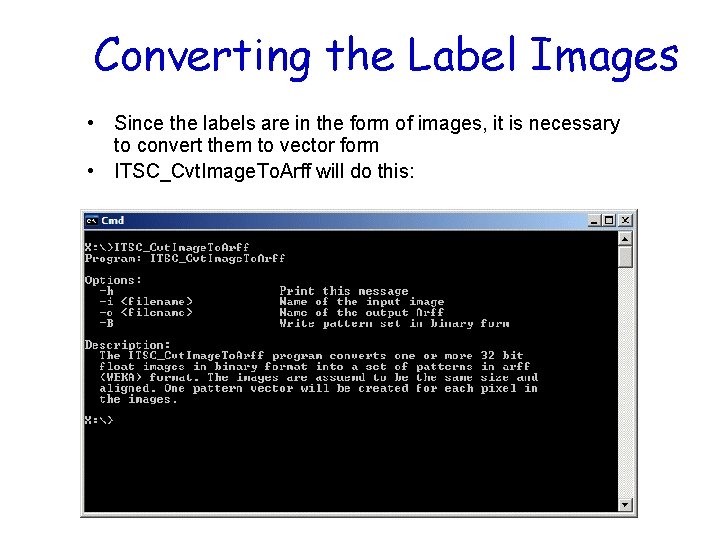
Converting the Label Images • Since the labels are in the form of images, it is necessary to convert them to vector form • ITSC_Cvt. Image. To. Arff will do this:

Converting ? ? ? • Since the labels are in the form of images, it is necessary to convert them to vector form • Consequences? • Do you save them? • Discussion?

Converting the Label Images • The labels can be converted to vector form using: ITSC_Cvt. Image. To. Arff –i lbl. bin –o lbl. arff -B • The –i argument specifies the input file name • The –o argument specifies the output file name • The –B argument tells the program to write the output file in binary form (default is ASCII)

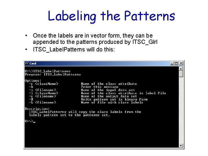
Labeling the Patterns • Once the labels are in vector form, they can be appended to the patterns produced by ITSC_Glrl • ITSC_Label. Patterns will do this:

Labeling the Patterns • The labels are assigned to patterns as follows: ITSC_Label. Patterns –i glrl. arff –c class –l lbl. bin –L lbl. arff –o all. arff –B • The –i argument specifies the input file name (patterns) • The –o argument specifies the output file name The –c argument • The –c argument specifies the name of the class attribute in the pattern set • The –l argument specifies the name of the label attribute in the label set • The –L argument specifies the name of the input label file • The –B argument tells the program to write the output file in binary form (default is ASCII)

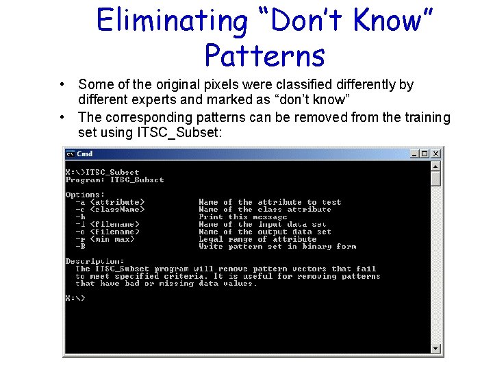
Eliminating “Don’t Know” Patterns • Some of the original pixels were classified differently by different experts and marked as “don’t know” • The corresponding patterns can be removed from the training set using ITSC_Subset:

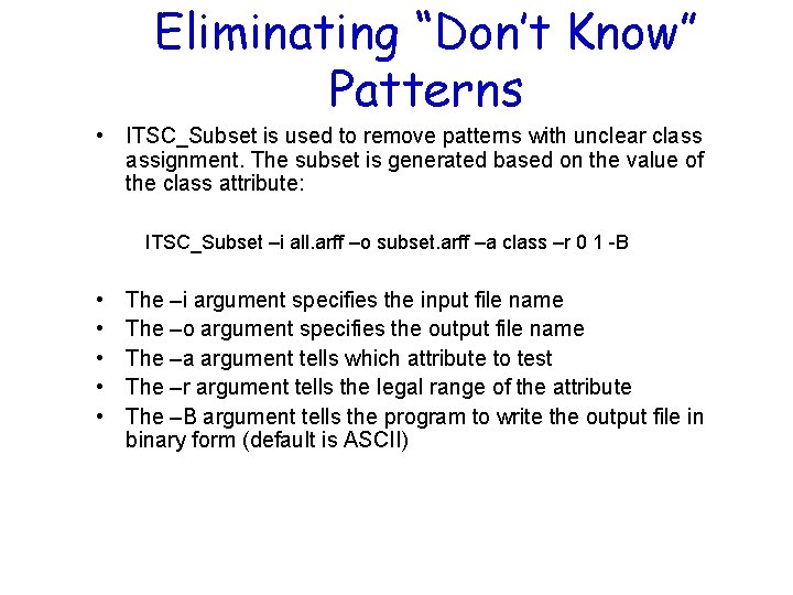
Eliminating “Don’t Know” Patterns • ITSC_Subset is used to remove patterns with unclear class assignment. The subset is generated based on the value of the class attribute: ITSC_Subset –i all. arff –o subset. arff –a class –r 0 1 -B • • • The –i argument specifies the input file name The –o argument specifies the output file name The –a argument tells which attribute to test The –r argument tells the legal range of the attribute The –B argument tells the program to write the output file in binary form (default is ASCII)

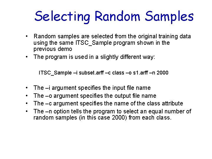
Selecting Random Samples • Random samples are selected from the original training data using the same ITSC_Sample program shown in the previous demo • The program is used in a slightly different way: ITSC_Sample –i subset. arff –c class –o s 1. arff –n 2000 • • The –i argument specifies the input file name The –o argument specifies the output file name The –c argument specifies the name of the class attribute The –n option tells the program to select an equal number of random samples (in this case 2000) from each class.

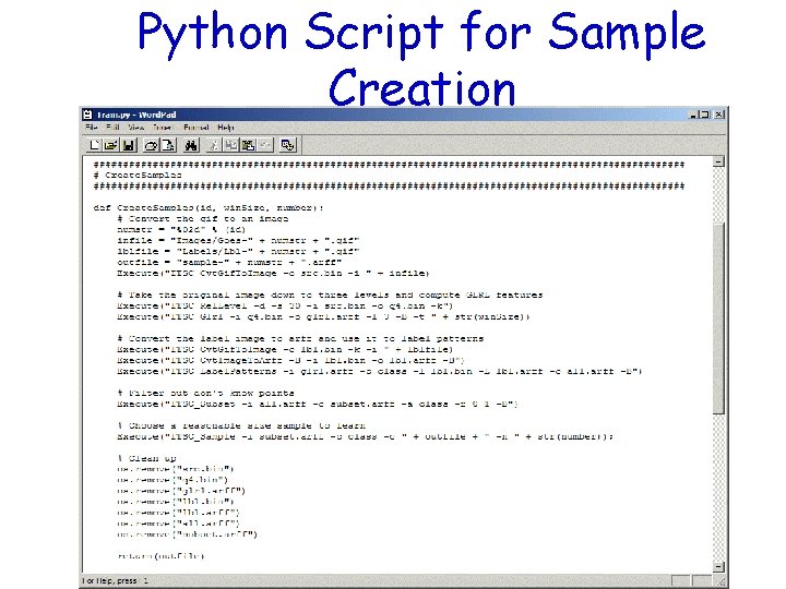
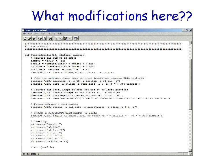
Python Script for Sample Creation

What modifications here? ?

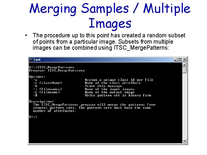
Merging Samples / Multiple Images • The procedure up to this point has created a random subset of points from a particular image. Subsets from multiple images can be combined using ITSC_Merge. Patterns:

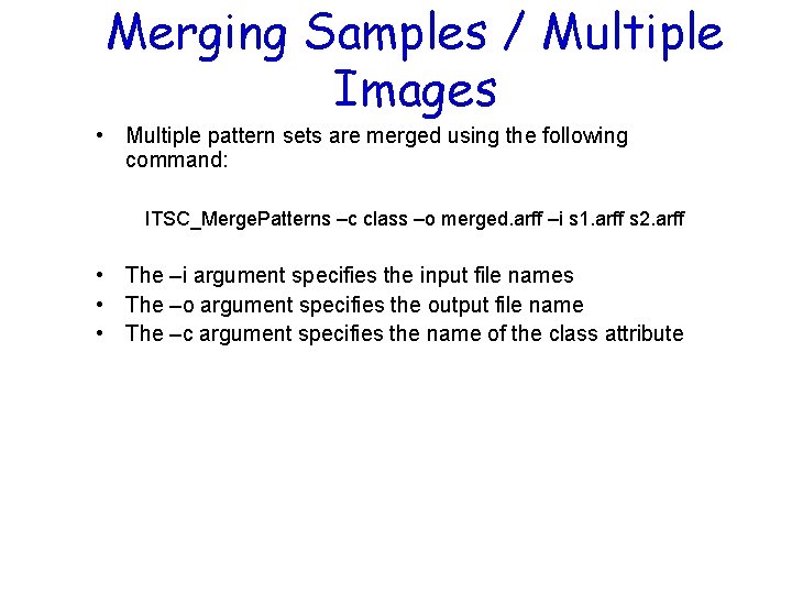
Merging Samples / Multiple Images • Multiple pattern sets are merged using the following command: ITSC_Merge. Patterns –c class –o merged. arff –i s 1. arff s 2. arff • The –i argument specifies the input file names • The –o argument specifies the output file name • The –c argument specifies the name of the class attribute

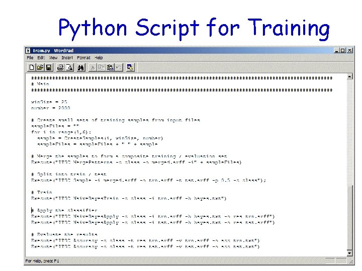
Python Script for Training

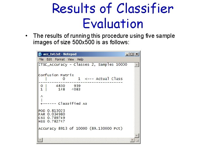
Results of Classifier Evaluation • The results of running this procedure using five sample images of size 500 x 500 is as follows:

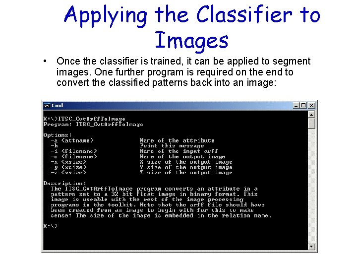
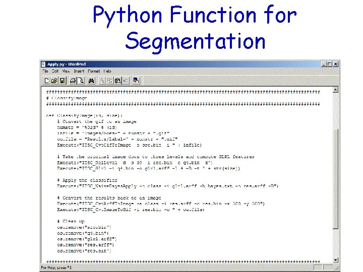
Applying the Classifier to Images • Once the classifier is trained, it can be applied to segment images. One further program is required on the end to convert the classified patterns back into an image:

Python Function for Segmentation

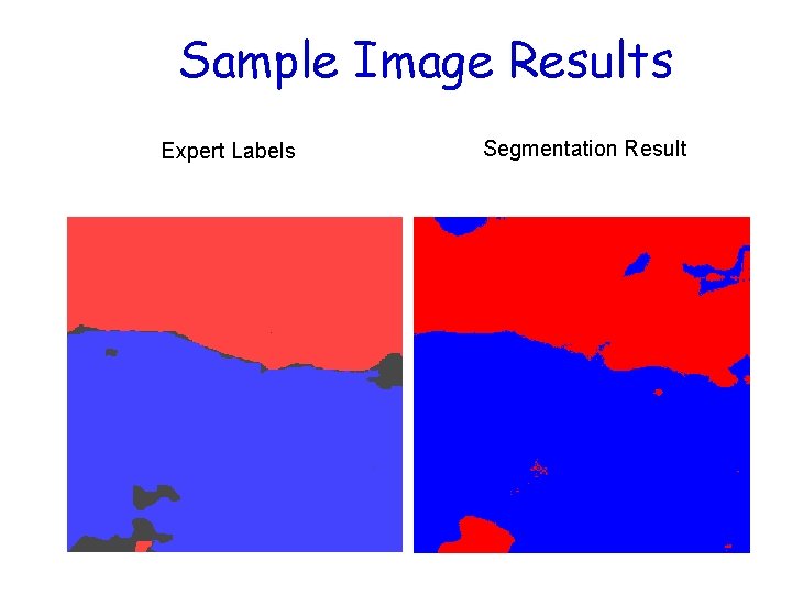
Sample Image Results Expert Labels Segmentation Result

Remarks • The procedure illustrated here is one specific example of ADa. M’s capabilities • There are many other classifiers, texture features and other tools that could be used for this problem • Since all of the algorithms of a particular type work in more or less the same way, the same general procedure could be used with other tools • DOWNLOAD the ADa. M Toolkit – http: //datamining. itsc. uah. edu/adam/

Numpy, scipy • http: //scikit-learn. org/stable/ • http: //orange. biolab. si 73

R • http: //www. rdatamining. com 74

Management • What did you learn? • Provenance elements? • How to deal with both?

What’s next 76

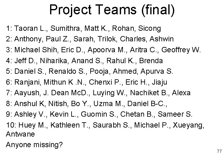
Project Teams (final) 1: Taoran L. , Sumithra, Matt K. , Rohan, Sicong 2: Anthony, Paul Z. , Sarah, Trilok, Charles, Ashwin 3: Michael Shih, Eric D. , Apoorva M. , Aritra C. , Geoffrey W. 4: Jeff D. , Niharika, Anand S. , Rahul K. , Brenda 5: Daniel S. , Renaldo S. , Pooja, Ahmed, Apurva S. 6: Ranjani, Mithun K. N. , Chenxi P. , Eric H. , Jiaju 7: Aayush, J. Dean Mc. D. , Luying W. , Nachiket B. , Alexa 8: Anshul K, Nitish, Bo Y. , Uzma M. , Daniel B-C. , 9: Ashley V. , Kevin L. , Guomin S. , Chetan B. , Sameer S. 10: Huey M. , Kathleen T. , Saurabh S. , Michael P. , Xueyang, Antwane Anyone missing? 77