Intro to Biostats Dave Nuber Definition of Population

Intro to Biostats Dave Nuber

Definition of Population and Sample • A population is a set of measurements of interest to the researcher • A sample is a subset of the population selected in such a way as to be representative of the population. • A sampling frame is the actual set of units from which a sample has been drawn: in the case of a simple random sample, all units from the sampling frame have an equal chance to be drawn and to occur in the sample. In the ideal case, the sampling frame should coincide with the population of interest.

Descriptive and Inferential Statistics • Descriptive Statistics provide enumeration, organization, and graphical representation of data. • Inferential Statistics provide a way to reach conclusions from samples (e. g. , to generalize from specific samples to populations). – An example would be to use a persons health status in a sample to draw inferences about underlying populations from which the sample is drawn.

Inferential Statistics • The objective of inferential statistics is to be able to draw an inference about a population parameter based on the information from a sample. – Estimating the prevalence of hypertension among Asian Indians living in New Jersey. – Hypothesis testing – testing the effectiveness of a new drug for reducing anxiety disorders.

Difference between surveys & experimental designs • Survey data represents observational data with respect to events over which there is no experimental control. – Assessing the association between stress and panic attacks. • Experimental designs involve the use of a research plan that imposes controls over the exposure or treatment. – Example: clinical trials.
 - units are independently selected one at a")
Sampling Methods • Random sampling (simple) - units are independently selected one at a time until the desired sample size is achieved. • Systematic sampling - if a sample size of n is desired, then the sampling fraction is n/N equivalent to 1/(N/n). The initial sampling unit, k, = N/n. Then chose the kth unit from the sampling frame. • Stratified sampling - divide the population in H distinct strata, such that the hth stratum has size Nh. A separate simple random sample of size nh is then selected for each stratum, resulting in a sampling fraction of nh/Nh for the hth group. • Cluster sampling - selecting a random sample of groups or clusters and then looking at all study units within the chosen groups. • Convenience sampling - simple sampling of the first n subjects in a population, may not be representative of the population.

Observational Studies • Retrospective Studies : gather past data from selected cases and controls to determine differences in the exposure to a suspected factor (cohort or case-control) • Prospective Studies: cohort studies in which healthy subjects are enrolled and then followed over a period of time to determine the frequency with which disease develops.

Variables in a study • • Independent Dependent Intermediate confounders

Independent Variable • The characteristic being observed or measured that is thought to influence the event or outcome (dependent variable) – The independent variable is not influenced by the event or outcome, but may cause it or may contribute to its variability.

Dependent Variables • A variable whose value is dependent on the effect of other variables in the study. – Also know as the outcome or response variable. – An event or outcome whose variability we are trying to explain or account for by the influence of the independent variables.

Intermediate Variable • A variable that occurs in a causal pathway from an independent to a dependent variable – intervening or mediating variables. – It produces variation in the dependent variable and is caused to vary by the independent variable. – Intermediate variables are associated with both the dependent and independent variables.

Confounding Variables • A factor that is itself a determinant of the outcome and that distorts the apparent effect of the study variable on the outcome. – Confounders may be unequally distributed among the exposed and the unexposed and thereby influence the apparent magnitude and even the direction of the effect.

Organizing Data • • • Frequency Table Frequency Histogram Relative Frequency Histogram Frequency Polygon Relative Frequency Polygon Bar Chart Pie Chart Stem-and-leaf display Box plot

Measures of Central Tendency • Mean - The arithmetic mean is computed by summing all the observations in the sample and dividing by the number of observations. • Median - Rank the values from smallest to highest, the median is the middle value • Mode - The observation that occurs most frequently.

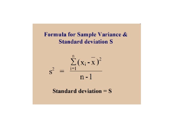
Measures of dispersion or variability • Range - the difference between the largest and smallest value in the data sample. • Variance = S 2 (next slide) • Standard deviation = s (next slide) • Coefficient of variation = s/X x 100%

Central Limit Theorem • Given a population of any nonnormal functional form with a mean µ and finite variance 2, the sampling distribution of , computed from sample size n from this population, will have mean µ and variance 2/n and will be approximately normally distributed when the sample size is large.

Normal Distribution

Empirical Rule • For a Normal Distribution – 68% of the values fall within one standard deviation from the mean – 95% of those values fall within two standard deviations from the mean – 99. 7% fall within three standard deviations from the mean

Statistical Tests

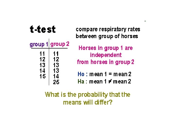
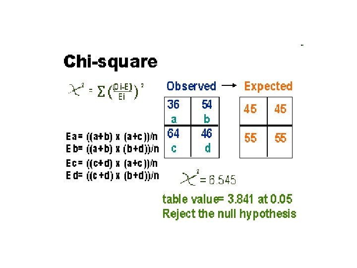
Commonly Statistical Tests • Correlation – linear relationships • T-test – associations between two means • Chi-square – association between proportions
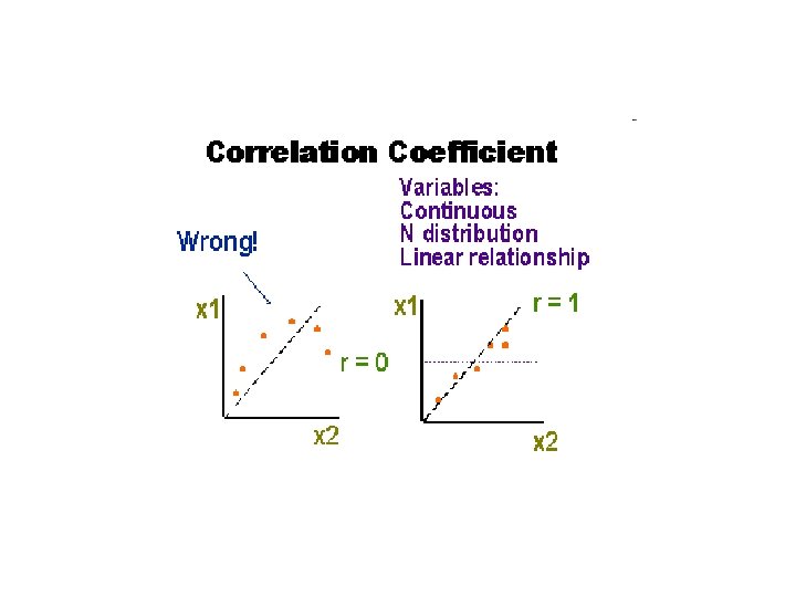

If you calculate the r 2 you may get an idea of the variability explained. r 2 = 0. 9382 = 0. 88 x 1 explaines 88% of the variability of x 2 (or x 2 explains 88% of the variability of x 1). Other unknown variables are explaining the rest.

One-way ANOVA • • A One-Way Analysis of Variance is a way to test the equality of two or more means at one time by using variances. Assumptions – The populations from which the samples were obtained must be normally or approximately normally distributed. – The samples must be independent. – The variances of the populations must be equal. • Hypotheses – The null hypothesis will be that all population means are equal, the alternative hypothesis is that at least one mean is different. – In the following, lower case letters apply to the individual samples and capital letters apply to the entire set collectively. That is, n is one of many sample sizes, but N is the total sample size. • Grand Mean – The grand mean of a set of samples is the total of all the data values divided by the total sample size. This requires that you have all of the sample data available to you, which is usually the case, but not always. It turns out that all that is necessary to find perform a oneway analysis of variance are the number of samples, the sample means, the sample variances, and the sample sizes. – Another way to find the grand mean is to find the weighted average of the sample means. The weight applied is the sample size.
 • Between Group Variation – The variation due to the interaction between")
ANOVA (cont’d) • Between Group Variation – The variation due to the interaction between the samples is denoted SS(B) for Sum of Squares Between groups. If the sample means are close to each other (and therefore the Grand Mean) this will be small. There are k samples involved with one data value for each sample (the sample mean), so there are k-1 degrees of freedom. – The variance due to the interaction between the samples is denoted MS(B) for Mean Square Between groups. This is the between group variation divided by its degrees of freedom. It is also denoted by. • Within Group Variation – The variation due to differences within individual samples, denoted SS(W) for Sum of Squares Within groups. Each sample is considered independently, no interaction between samples is involved. The degrees of freedom is equal to the sum of the individual degrees of freedom for each sample. Since each sample has degrees of freedom equal to one less than their sample sizes, and there are k samples, the total degrees of freedom is k less than the total sample size: df = N - k. – The variance due to the differences within individual samples is denoted MS(W) for Mean Square Within groups. This is the within group variation divided by its degrees of freedom. It is also denoted by. It is the weighted average of the variances (weighted with the degrees of freedom). • F test statistic – Recall that a F variable is the ratio of two independent chi-square variables divided by their respective degrees of freedom. Also recall that the F test statistic is the ratio of two sample variances, well, it turns out that's exactly what we have here. The F test statistic is found by dividing the between group variance by the within group variance. The degrees of freedom for the numerator are the degrees of freedom for the between group (k-1) and the degrees of freedom for the denominator are the degrees of freedom for the within group (N-k).
 k-1 SS(B ) -----k 1 Within SS(W)")
Summary Table SS df MS Between SS(B) k-1 SS(B ) -----k 1 Within SS(W) N-k SS( W) -----N-k F MS(B) ------MS(W). SS(W) + SS(B). . its degrees of freedom, and the F Notice. Total that each Mean Square is just the. N-1 Sum of Squares divided by value is the ratio of the mean squares. Do not put the largest variance in the numerator, always divide the between variance by the within variance. If the between variance is smaller than the within variance, then the means are really close to each other and you will fail to reject the claim that they are all equal. The degrees of freedom of the F-test are in the same order they appear in the table.

Decision Rule • The decision will be to reject the null hypothesis if the test statistic from the table is greater than the F critical value with k-1 numerator and N-k denominator degrees of freedom. • If the decision is to reject the null, then at least one of the means is different. However, the ANOVA does not tell you where the difference lies. For this, you need another test, either the Scheffe' or Tukey test.

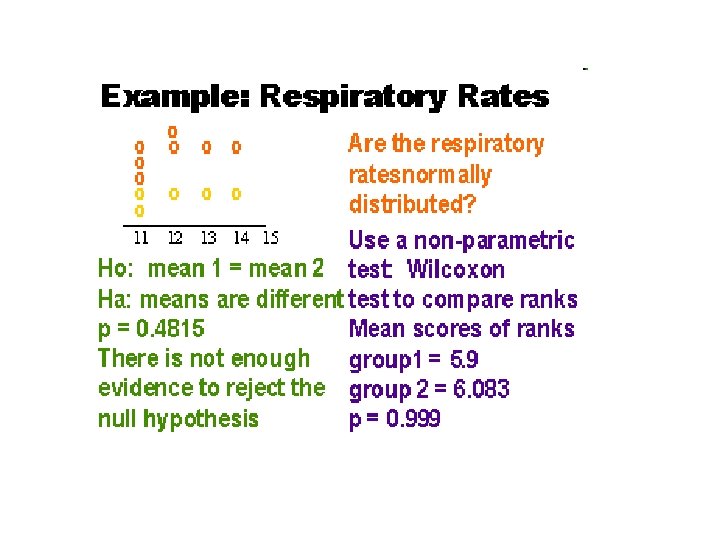
Mann-Whitney U test • Observations are ranked in order of magnitude with n 1 n 2 pairs of xiyj such that: – UXY is the number of pairs for which xi < yj and – UYX is the number of pairs for which xi > yj. – Any pairs for which xi = yj counts 1/2 of a unit towards both UXY and UYX. Either statistic may be used. • For instance, UYX must lie between 0 and n 1 n 2. • Null hypothesis its expectation is 1/2 n 1 n 2. If greater than 1/2 n 1 n 2, then x tends to be greater than y

Wilcoxon’s Rank Sum • T 1 is the sum of the ranks of the xis. • T 2 is the sum of the ranks of the yjs. – Low values assume low ranks (rank 1 is alloted to the smallest values). Any group of tied ranks is allotted the midrank of the group. • The smallest value which T 1 can take arises when all the xs are less than all the ys. – Then T 1 = 1/2 n 1(n 1 + 1). • The maximum value which T 1 can take arises when all the xs are greater than all the ys. – The T 1 = n 1 n 2 + 1/2 n 1(n 1 + 1). • Null expectation of T 1 is 1/2 n 1(n 1 + n 2 + 1).

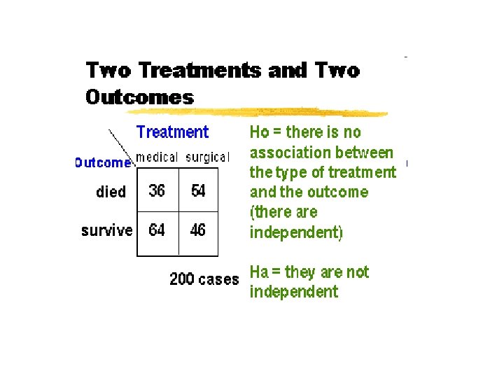
Fisher’s exact test • The test for association in a 2 x 2 table that is based on the exact hypergeometric distribution of the frequencies in the table. • Data is arranged in a 2 x 2 contingency table. – Arrange frequencies such that A > B and choose the characteristic of interest so that a/A > b/B Sample With Characteristic Without Characteristic Total 1 a A-a A 2 b B-b B Total a+b A+B+a+b A+B

Fisher’s Exact Test Assumptions • Data consist of A sample observations from population 1 and B sample observations from population 2. • The samples are random and independent • Each observation can be categorized as one of two mutually exclusive types.

Hypotheses • Two sided test – HO: the proportion with the characteristic of interest is the same in both populations (p 1 = p 2) – HA: the proportion with the characteristic of interest is not the same in both populations (p 1 p 2) • One sided test – HO: the proportion with the characteristic of interest in population 1 is less than or the same in population 2 (p 1 p 2) – HA: the proportion with the characteristic of interest is not the same in both populations (p 1 > p 2) • Test Statistic - b, the number in sample 2 with the characteristic of interest.

Mc. Nemar’s test • Paired samples for counts • Each observation in the first group has a corresponding observation in the second group.

Mc. Nemar’s Example MI Diabetes Yes No Total Yes 46 25 71 No 98 119 217 Total 144 288
 NO MI MI Yes No Total Yes 9 37 46")
Mc. Nemar’s Example (cont’d) NO MI MI Yes No Total Yes 9 37 46 No 16 82 96 Total 25 119 144

Mc. Nemar’s Ex - Hypothesis Test • HO: there is no association between diabetes and acute MI • HA: there is an association between diabetes and acute MI • How do we do this test? – Focus on the discordant pairs, the pairs of responses where someone has diabetes is paired with someone who does not.

Mc. Nemar’s Test Statistic ‘r = number of pairs in which someone with MI has diabetes and the other person without MI does not have diabetes ‘s = number of pairs in which someone without MI is a diabetic but the other person with MI is not diabetic. X 2 = [ r - s ]-1]2 / (r + s) The ratio is approximately Chi-square distribution with 1 degree of freedom.
![Mc. Nemar’s Example X 2 = [ 37 - 16 ]-1]2 / (37 +](http://slidetodoc.com/presentation_image_h2/41cf494bdc1e90fc816504d7501fe461/image-45.jpg "Mc. Nemar’s Example X 2 = [ 37 - 16 ]-1]2 / (37 +")
Mc. Nemar’s Example X 2 = [ 37 - 16 ]-1]2 / (37 + 16) X 2 = [21 -1]2 / (53) X 2 = 7. 55 The Chi-Sq distribution with 1 df, 0. 001 < p < 0. 01. We reject the HO at the. 05 level in favor of the HA, concluding that among Navajos there is a difference between people who have MI and those who do not, those with MI are more likely to have diabetes than those without MI who have been matched on age and gender.
2 n")
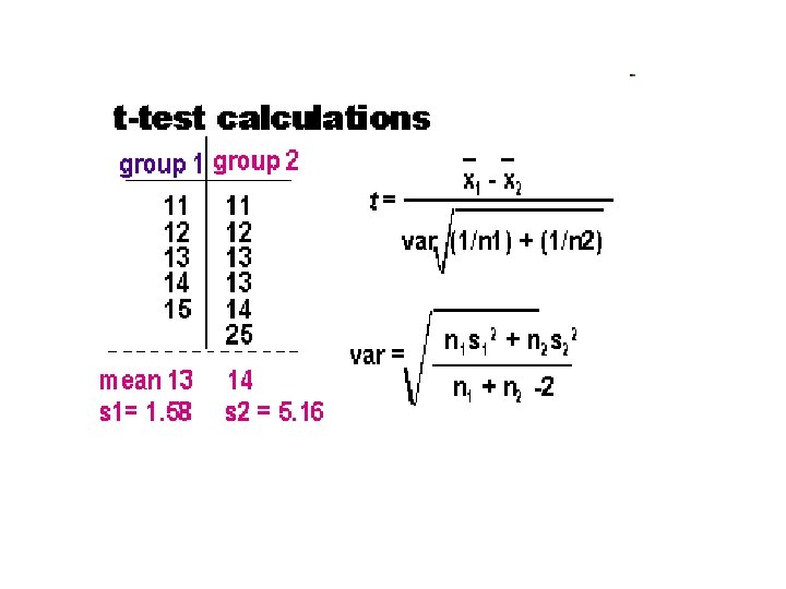
Paired t-test - equal variances s 12 = ∑ (x - x-bar 1)2 n 1 - 1 s 22 = ∑ (x - x-bar 2)2 n 2 - 1 s 2 = (n 1 -1)s 12 + (n 2 - 1)s 22 (n 1 - 1) + (n 2 - 1) = ∑ (x-xbar 1)2 + ∑ (x - xbar 2)2 n 1 + n 2 - 2
 = [ s")
Paired t-test - equal variances SE (X-bar 1 - X-bar 2) = [ s 2 (1/n 1 + 1/n 2)] t= X-bar 1 - X-bar 2 SE (X-bar 1 - X-bar 2) Which follows a t- distribution win n 1+n 2 -2 df Conf Limit is given by: X-bar 1 -X-bar 2 ± tv, . 05 SE(X-bar 1 - X-bar 2) With v = n 1+n 2 -2
 = [ (s")
Paired t-test - unequal variances SE (X-bar 1 - X-bar 2) = [ (s 12/n 1) + (s 22/n 2)] d= X-bar 1 - X-bar 2 √ (s 12/n 1) + (s 22/n 2) Which follows a normal distribution when n 1 and n 2 are sufficiently large Conf Limit is given by: X-bar 1 -X-bar 2 ± Z. 05 SE(X-bar 1 - X-bar 2)

Error Rates True Relationship Hypothesis Chosen HO HO Correct Decision HA HA False Negative Decision (Type II error) False Positive Correct Decision (Type I Decision error)

Probabilities of outcomes of hypothesis testing True Relationship Hypothesis Chosen HO HA HO 1 - HA 1 -
2 2 2")
Sample size calculation n 2 (Z 1 -a + Z 1 -b)2 2 2
- Slides: 51