Intro ANN Fuzzy Systems Lecture 14 MLP VI

Intro. ANN & Fuzzy Systems Lecture 14. MLP (VI): Model Selection (C) 2001 by Yu Hen Hu

Intro. ANN & Fuzzy Systems Outline • Universal approximation property • Network structure selection • Structural Design of MLP – Dynamic and Static Growing Methods – Dynamic and Static Pruning Methods • Batch Learning Methods (C) 2001 by Yu Hen Hu 2

Intro. ANN & Fuzzy Systems Configuration of MLP • The choice of number of hidden nodes is – problem and data dependent; – even the optimal number is given, training may take long and finding optimal weights may be difficult. • Methods for changing the number of hidden nodes dynamically are available, but not widely used. Two approaches: Growing vs. pruning. (C) 2001 by Yu Hen Hu 3

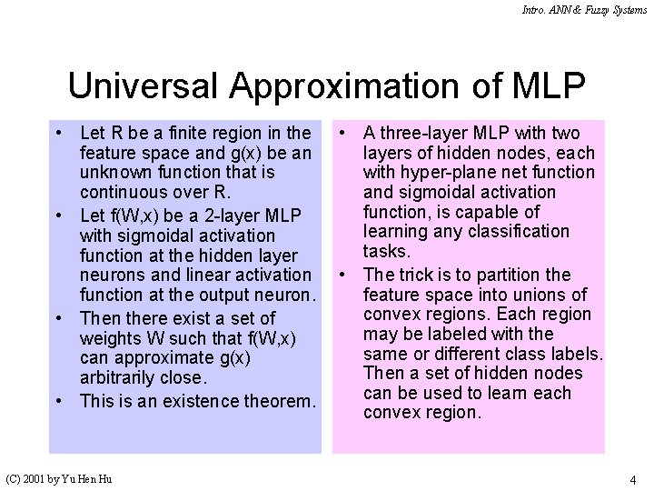
Intro. ANN & Fuzzy Systems Universal Approximation of MLP • Let R be a finite region in the • A three-layer MLP with two feature space and g(x) be an layers of hidden nodes, each unknown function that is with hyper-plane net function continuous over R. and sigmoidal activation function, is capable of • Let f(W, x) be a 2 -layer MLP learning any classification with sigmoidal activation tasks. function at the hidden layer neurons and linear activation • The trick is to partition the function at the output neuron. feature space into unions of convex regions. Each region • Then there exist a set of may be labeled with the weights W such that f(W, x) same or different class labels. can approximate g(x) Then a set of hidden nodes arbitrarily close. can be used to learn each • This is an existence theorem. convex region. (C) 2001 by Yu Hen Hu 4

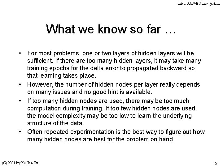
Intro. ANN & Fuzzy Systems What we know so far … • For most problems, one or two layers of hidden layers will be sufficient. If there are too many hidden layers, it may take many training epochs for the delta error to propagated backward so that learning takes place. • However, the number of hidden nodes per layer really depends on many issues and no good hint is available. • If too many hidden nodes are used, there may be too much computation during training. If too few hidden nodes are used, the model complexity may be too low to learn the underlying structure of the data. • Often repeated experimentation is the best way to figure out how many hidden nodes are best for the problem on hand. (C) 2001 by Yu Hen Hu 5

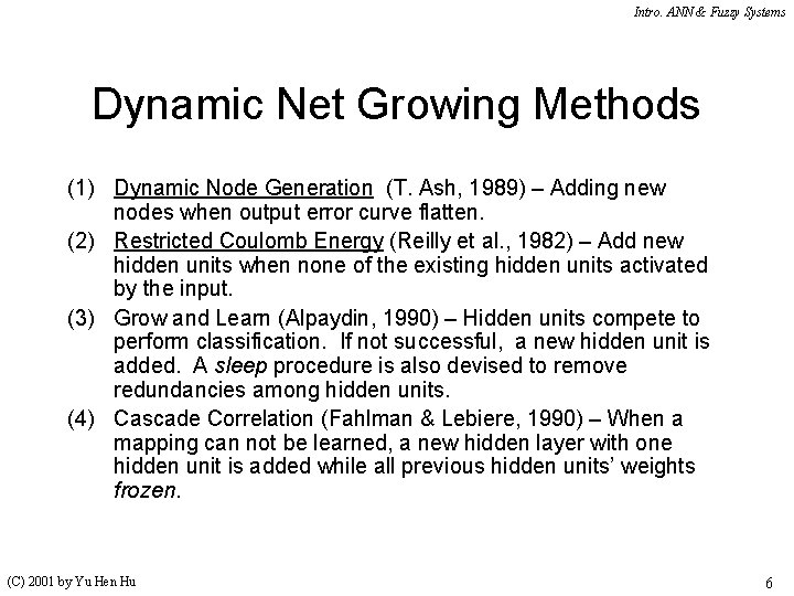
Intro. ANN & Fuzzy Systems Dynamic Net Growing Methods (1) Dynamic Node Generation (T. Ash, 1989) – Adding new nodes when output error curve flatten. (2) Restricted Coulomb Energy (Reilly et al. , 1982) – Add new hidden units when none of the existing hidden units activated by the input. (3) Grow and Learn (Alpaydin, 1990) – Hidden units compete to perform classification. If not successful, a new hidden unit is added. A sleep procedure is also devised to remove redundancies among hidden units. (4) Cascade Correlation (Fahlman & Lebiere, 1990) – When a mapping can not be learned, a new hidden layer with one hidden unit is added while all previous hidden units’ weights frozen. (C) 2001 by Yu Hen Hu 6

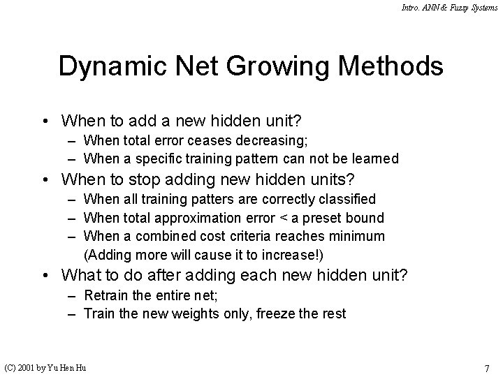
Intro. ANN & Fuzzy Systems Dynamic Net Growing Methods • When to add a new hidden unit? – When total error ceases decreasing; – When a specific training pattern can not be learned • When to stop adding new hidden units? – When all training patters are correctly classified – When total approximation error < a preset bound – When a combined cost criteria reaches minimum (Adding more will cause it to increase!) • What to do after adding each new hidden unit? – Retrain the entire net; – Train the new weights only, freeze the rest (C) 2001 by Yu Hen Hu 7

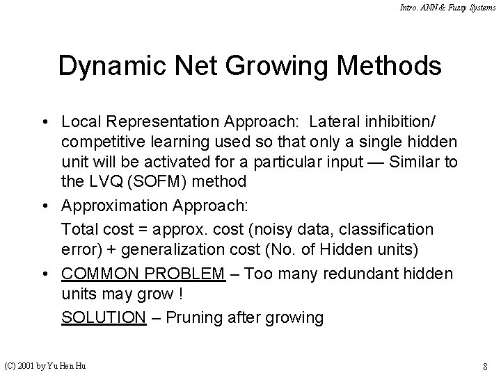
Intro. ANN & Fuzzy Systems Dynamic Net Growing Methods • Local Representation Approach: Lateral inhibition/ competitive learning used so that only a single hidden unit will be activated for a particular input — Similar to the LVQ (SOFM) method • Approximation Approach: Total cost = approx. cost (noisy data, classification error) + generalization cost (No. of Hidden units) • COMMON PROBLEM – Too many redundant hidden units may grow ! SOLUTION – Pruning after growing (C) 2001 by Yu Hen Hu 8

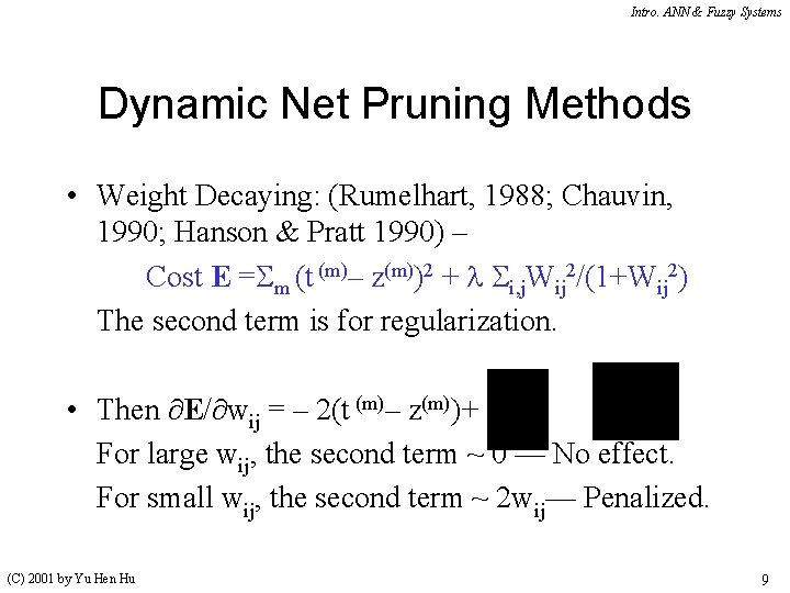
Intro. ANN & Fuzzy Systems Dynamic Net Pruning Methods • Weight Decaying: (Rumelhart, 1988; Chauvin, 1990; Hanson & Pratt 1990) – Cost E = m (t (m)– z(m))2 + l i, j. Wij 2/(1+Wij 2) The second term is for regularization. • Then E/ wij = – 2(t (m)– z(m))+ l For large wij, the second term ~ 0 –– No effect. For small wij, the second term ~ 2 wij–– Penalized. (C) 2001 by Yu Hen Hu 9

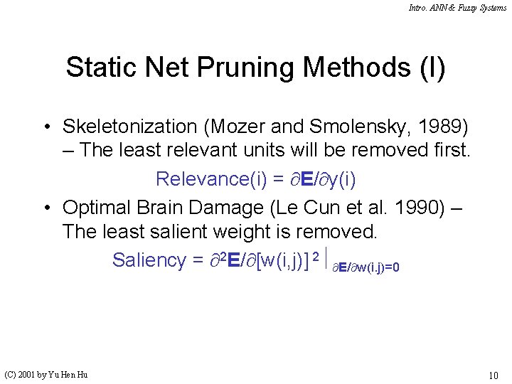
Intro. ANN & Fuzzy Systems Static Net Pruning Methods (I) • Skeletonization (Mozer and Smolensky, 1989) – The least relevant units will be removed first. Relevance(i) = E/ y(i) • Optimal Brain Damage (Le Cun et al. 1990) – The least salient weight is removed. Saliency = 2 E/ [w(i, j)] 2 E/ w(i. j)=0 (C) 2001 by Yu Hen Hu 10

Intro. ANN & Fuzzy Systems Static Net Pruning Methods (II) • Hidden Unit Reduction Method (Hu et. al 1990) –The set of hidden units whose outputs are most independent are retained. • Frobinius Norm Approximation Method (Kung & Hu 1990) – Hidden units whose output best approximate the activation of the trained network are retained. (C) 2001 by Yu Hen Hu 11

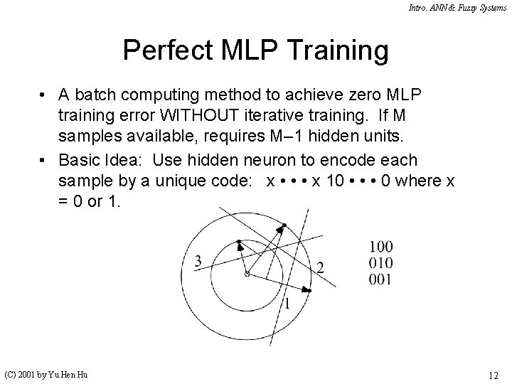
Intro. ANN & Fuzzy Systems Perfect MLP Training • A batch computing method to achieve zero MLP training error WITHOUT iterative training. If M samples available, requires M– 1 hidden units. • Basic Idea: Use hidden neuron to encode each sample by a unique code: x • • • x 10 • • • 0 where x = 0 or 1. (C) 2001 by Yu Hen Hu 12

Intro. ANN & Fuzzy Systems Perfect Training Algorithm 1. Sort all input x(k); 1 k K such that ||x(k)|| ||x(k+1)||. 2. For k = 1 to K– 1 Do Add k-th neuron with weight vector wk, bias qk s. t. wk = x(k), k= –(1/2)[||x(k)|| + max([x(k)] Tx(k'); k' > k)]. 3. Compute hidden node output matrix YKx(K-1) for all inputs. Y matrix has 1 along its main diagonal. 4. Compute weights and bias of output neurons as: [q W] = [1 Y] 1 f 1(T) T: target vector (all inputs), f 1( ): inverse activation function. (C) 2001 by Yu Hen Hu 13

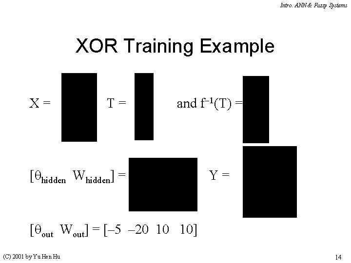
Intro. ANN & Fuzzy Systems XOR Training Example X= T= and f 1(T) = [ hidden Whidden] = Y= [ out Wout] = [– 5 – 20 10 10] (C) 2001 by Yu Hen Hu 14

Intro. ANN & Fuzzy Systems XOR Result and Pruning Left two neurons have the same output as X, hence can be eliminated w/o affecting the result. (C) 2001 by Yu Hen Hu 15