Intertemporal Consumption Choice Economics 101 In ECO 100

Inter-temporal Consumption Choice

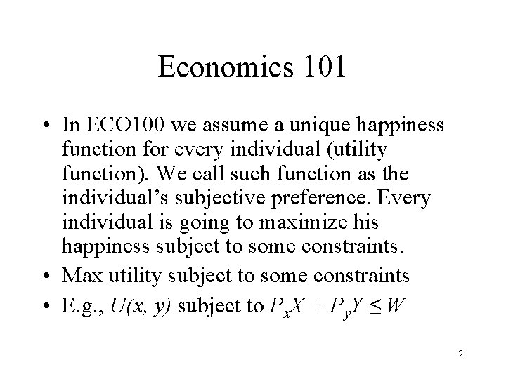
Economics 101 • In ECO 100 we assume a unique happiness function for every individual (utility function). We call such function as the individual’s subjective preference. Every individual is going to maximize his happiness subject to some constraints. • Max utility subject to some constraints • E. g. , U(x, y) subject to Px. X + Py. Y ≤ W 2

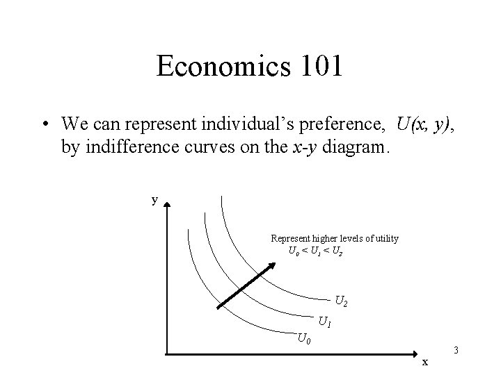
Economics 101 • We can represent individual’s preference, U(x, y), by indifference curves on the x-y diagram. y Represent higher levels of utility U 0 < U 1 < U 2 U 1 U 0 x 3

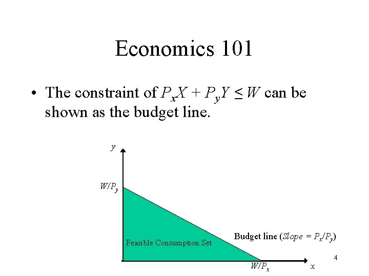
Economics 101 • The constraint of Px. X + Py. Y ≤ W can be shown as the budget line. y W/Py Feasible Consumption Set Budget line (Slope = Px/Py) W/Px x 4

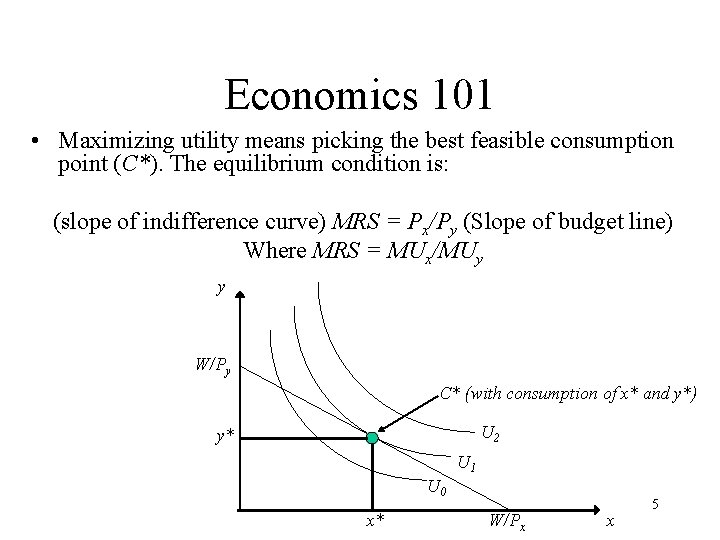
Economics 101 • Maximizing utility means picking the best feasible consumption point (C*). The equilibrium condition is: (slope of indifference curve) MRS = Px/Py (Slope of budget line) Where MRS = MUx/MUy y W/Py C* (with consumption of x* and y*) U 2 y* U 1 U 0 x* W/Px x 5

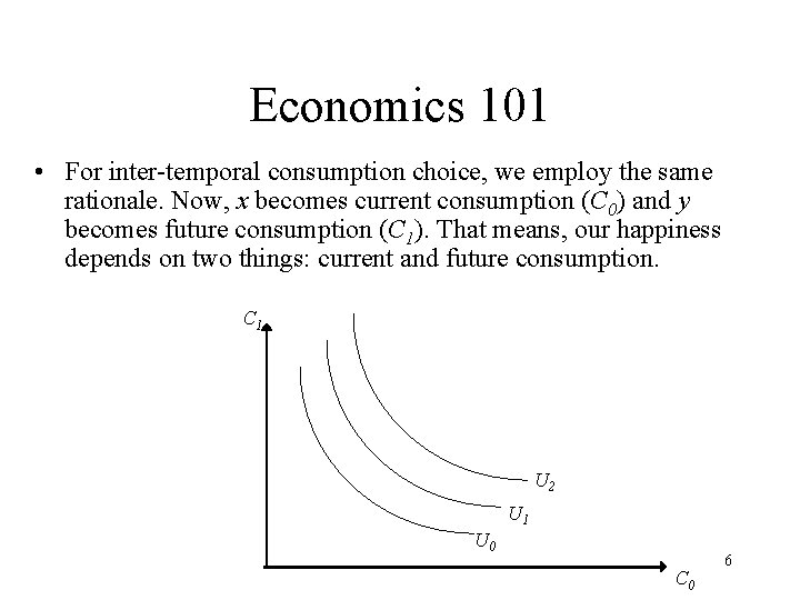
Economics 101 • For inter-temporal consumption choice, we employ the same rationale. Now, x becomes current consumption (C 0) and y becomes future consumption (C 1). That means, our happiness depends on two things: current and future consumption. C 1 U 2 U 1 U 0 C 0 6

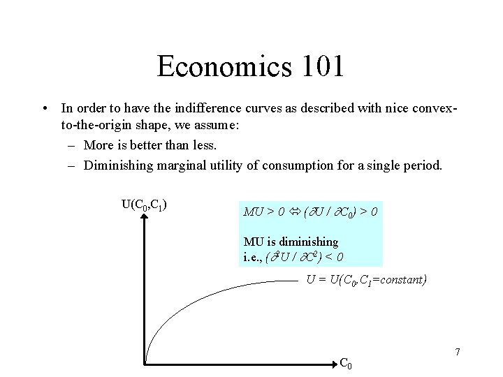
Economics 101 • In order to have the indifference curves as described with nice convexto-the-origin shape, we assume: – More is better than less. – Diminishing marginal utility of consumption for a single period. U(C 0, C 1) MU > 0 ( U / C 0) > 0 MU is diminishing i. e. , ( 2 U / C 2) < 0 U = U(C 0, C 1=constant) C 0 7

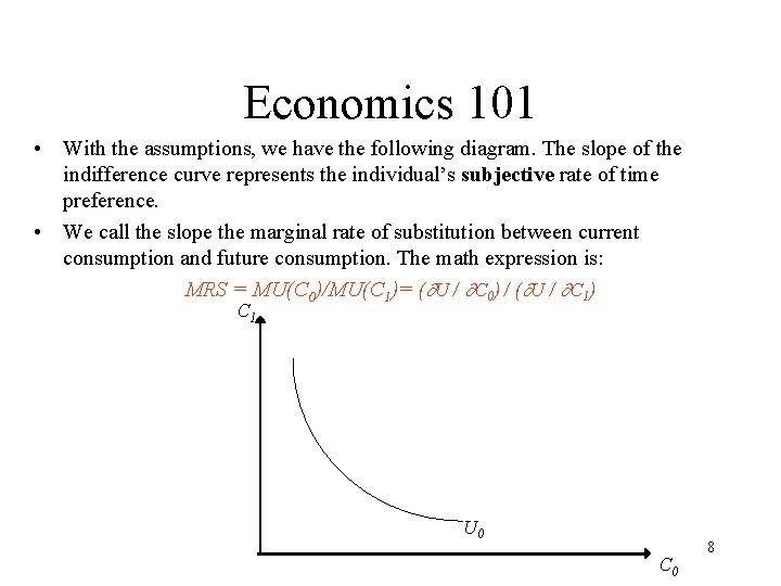
Economics 101 • With the assumptions, we have the following diagram. The slope of the indifference curve represents the individual’s subjective rate of time preference. • We call the slope the marginal rate of substitution between current consumption and future consumption. The math expression is: MRS = MU(C 0)/MU(C 1)= ( U / C 0) / ( U / C 1) C 1 U 0 C 0 8

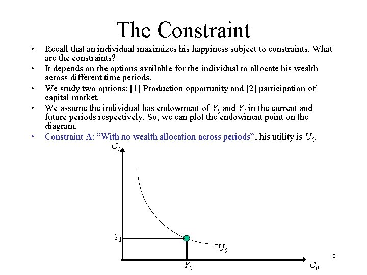
The Constraint • • • Recall that an individual maximizes his happiness subject to constraints. What are the constraints? It depends on the options available for the individual to allocate his wealth across different time periods. We study two options: [1] Production opportunity and [2] participation of capital market. We assume the individual has endowment of Y 0 and Y 1 in the current and future periods respectively. So, we can plot the endowment point on the diagram. Constraint A: “With no wealth allocation across periods”, his utility is U 0. C 1 Y 1 U 0 Y 0 C 0 9

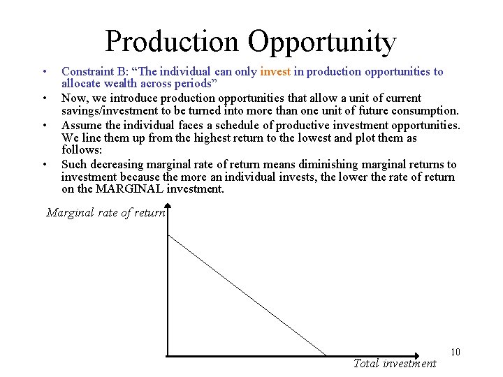
Production Opportunity • • Constraint B: “The individual can only invest in production opportunities to allocate wealth across periods” Now, we introduce production opportunities that allow a unit of current savings/investment to be turned into more than one unit of future consumption. Assume the individual faces a schedule of productive investment opportunities. We line them up from the highest return to the lowest and plot them as follows: Such decreasing marginal rate of return means diminishing marginal returns to investment because the more an individual invests, the lower the rate of return on the MARGINAL investment. Marginal rate of return Total investment 10

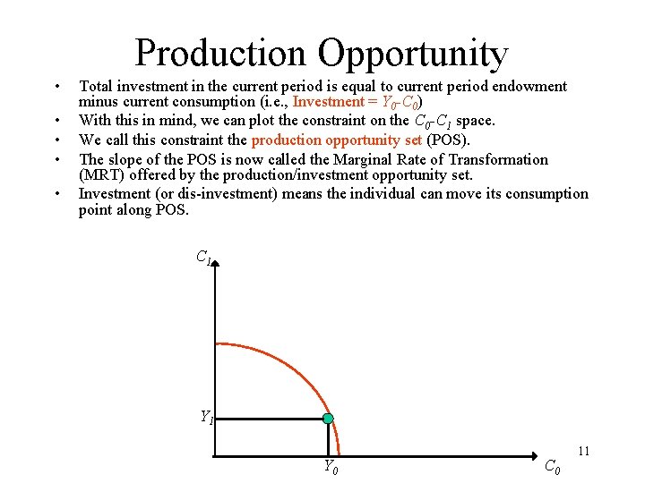
Production Opportunity • • • Total investment in the current period is equal to current period endowment minus current consumption (i. e. , Investment = Y 0 -C 0) With this in mind, we can plot the constraint on the C 0 -C 1 space. We call this constraint the production opportunity set (POS). The slope of the POS is now called the Marginal Rate of Transformation (MRT) offered by the production/investment opportunity set. Investment (or dis-investment) means the individual can move its consumption point along POS. C 1 Y 0 C 0 11

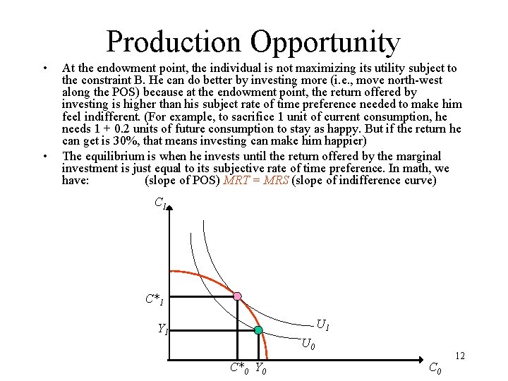
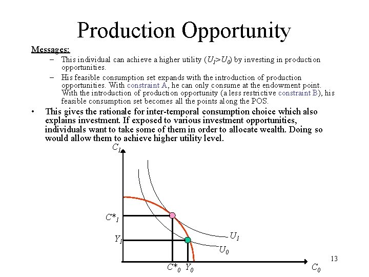
Production Opportunity • • At the endowment point, the individual is not maximizing its utility subject to the constraint B. He can do better by investing more (i. e. , move north-west along the POS) because at the endowment point, the return offered by investing is higher than his subject rate of time preference needed to make him feel indifferent. (For example, to sacrifice 1 unit of current consumption, he needs 1 + 0. 2 units of future consumption to stay as happy. But if the return he can get is 30%, that means investing can make him happier) The equilibrium is when he invests until the return offered by the marginal investment is just equal to its subjective rate of time preference. In math, we have: (slope of POS) MRT = MRS (slope of indifference curve) C 1 C*1 U 1 Y 1 U 0 C*0 Y 0 C 0 12

Production Opportunity Messages: – This individual can achieve a higher utility (U 1>U 0) by investing in production opportunities. – His feasible consumption set expands with the introduction of production opportunities. With constraint A, he can only consume at the endowment point. With the introduction of production opportunity (a less restrictive constraint B), his feasible consumption set becomes all the points along the POS. • This gives the rationale for inter-temporal consumption choice which also explains investment. If exposed to various investment opportunities, individuals want to take some of them in order to allocate wealth. Doing so would allow them to achieve higher utility level. C 1 C*1 U 1 Y 1 U 0 C*0 Y 0 C 0 13

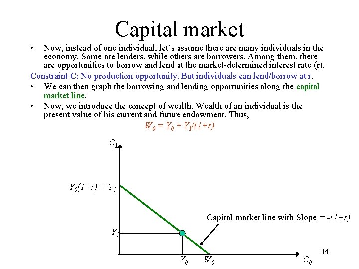
Capital market • Now, instead of one individual, let’s assume there are many individuals in the economy. Some are lenders, while others are borrowers. Among them, there are opportunities to borrow and lend at the market-determined interest rate (r). Constraint C: No production opportunity. But individuals can lend/borrow at r. • We can then graph the borrowing and lending opportunities along the capital market line. • Now, we introduce the concept of wealth. Wealth of an individual is the present value of his current and future endowment. Thus, W 0 = Y 0 + Y 1/(1+r) C 1 Y 0(1+r) + Y 1 Capital market line with Slope = -(1+r) Y 1 Y 0 W 0 C 0 14

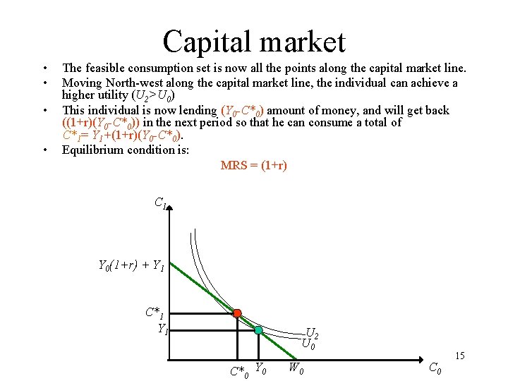
Capital market • • The feasible consumption set is now all the points along the capital market line. Moving North-west along the capital market line, the individual can achieve a higher utility (U 2>U 0) This individual is now lending (Y 0 -C*0) amount of money, and will get back ((1+r)(Y 0 -C*0)) in the next period so that he can consume a total of C*1= Y 1+(1+r)(Y 0 -C*0). Equilibrium condition is: MRS = (1+r) C 1 Y 0(1+r) + Y 1 C*1 Y 1 U 2 U 0 C*0 Y 0 W 0 C 0 15

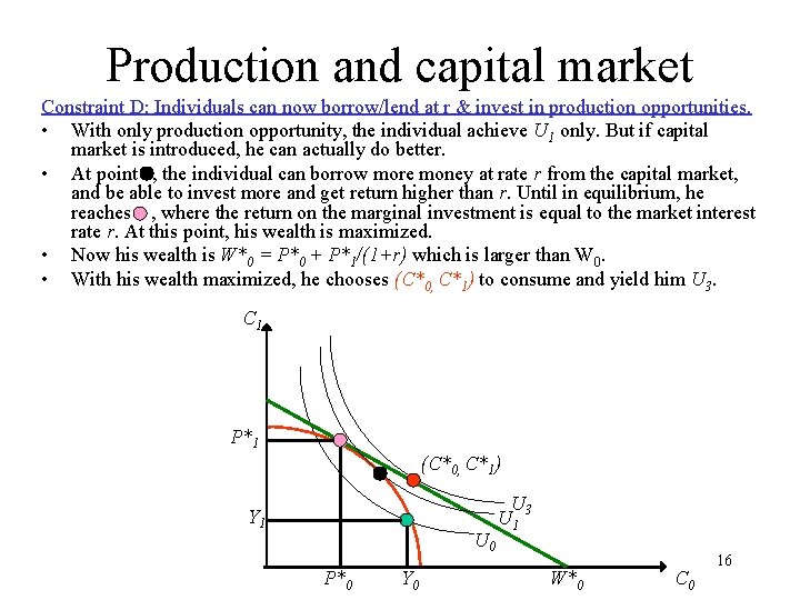
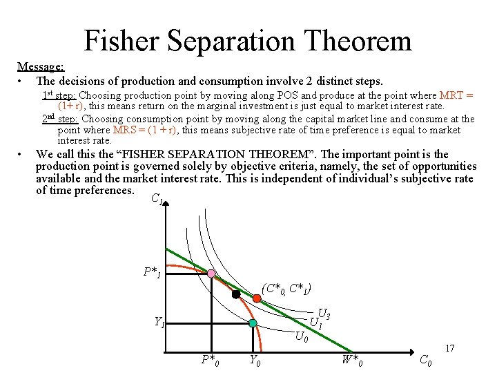
Production and capital market Constraint D: Individuals can now borrow/lend at r & invest in production opportunities. • With only production opportunity, the individual achieve U 1 only. But if capital market is introduced, he can actually do better. • At point , the individual can borrow more money at rate r from the capital market, and be able to invest more and get return higher than r. Until in equilibrium, he reaches , where the return on the marginal investment is equal to the market interest rate r. At this point, his wealth is maximized. • Now his wealth is W*0 = P*0 + P*1/(1+r) which is larger than W 0. • With his wealth maximized, he chooses (C*0, C*1) to consume and yield him U 3. C 1 P*1 (C*0, C*1) Y 1 U 0 P*0 Y 0 U 3 U 1 W*0 C 0 16

Fisher Separation Theorem Message: • The decisions of production and consumption involve 2 distinct steps. 1 st step: Choosing production point by moving along POS and produce at the point where MRT = (1+ r), this means return on the marginal investment is just equal to market interest rate. 2 nd step: Choosing consumption point by moving along the capital market line and consume at the point where MRS = (1 + r), this means subjective rate of time preference is equal to market interest rate. • We call this the “FISHER SEPARATION THEOREM”. The important point is the production point is governed solely by objective criteria, namely, the set of opportunities available and the market interest rate. This is independent of individual’s subjective rate of time preferences. C 1 P*1 (C*0, C*1) Y 1 U 0 P*0 Y 0 U 3 U 1 W*0 C 0 17

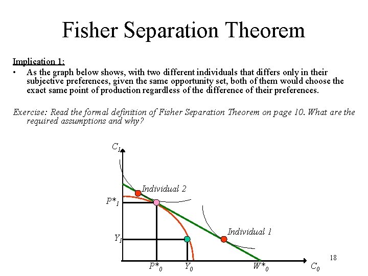
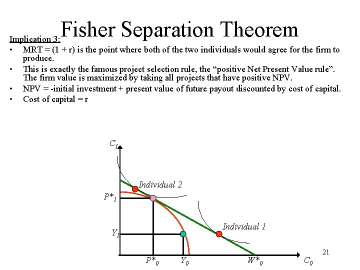
Fisher Separation Theorem Implication 1: • As the graph below shows, with two different individuals that differs only in their subjective preferences, given the same opportunity set, both of them would choose the exact same point of production regardless of the difference of their preferences. Exercise: Read the formal definition of Fisher Separation Theorem on page 10. What are the required assumptions and why? C 1 Individual 2 P*1 Individual 1 Y 1 P*0 Y 0 W*0 C 0 18

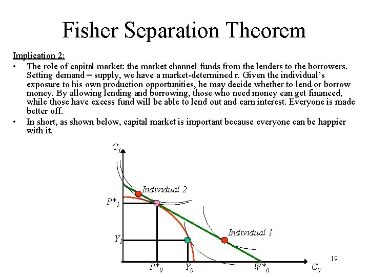
Fisher Separation Theorem Implication 2: • The role of capital market: the market channel funds from the lenders to the borrowers. Setting demand = supply, we have a market-determined r. Given the individual’s exposure to his own production opportunities, he may decide whether to lend or borrow money. By allowing lending and borrowing, those who need money can get financed, while those have excess fund will be able to lend out and earn interest. Everyone is made better off. • In short, as shown below, capital market is important because everyone can be happier with it. C 1 Individual 2 P*1 Individual 1 Y 1 P*0 Y 0 W*0 C 0 19

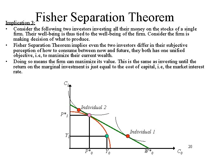
Fisher Separation Theorem Implication 3: • Consider the following two investors investing all their money on the stocks of a single firm. Their well-being is thus tied to the well-being of the firm. Consider the firm is making decision of what to produce. • Fisher Separation Theorem implies even the two investors differ in their subjective perception of how to consume between now and future, they both has one unified objective, i. e, to maximize their current wealth. • Doing so means the firm can maximize its value. This is the same as investing until the return on the marginal investment is just equal to the cost of capital, i. e, the market interest rate. C 1 Individual 2 P*1 Individual 1 Y 1 P*0 Y 0 W*0 C 0 20

Fisher Separation Theorem Implication 3: • MRT = (1 + r) is the point where both of the two individuals would agree for the firm to produce. • This is exactly the famous project selection rule, the “positive Net Present Value rule”. The firm value is maximized by taking all projects that have positive NPV. • NPV = -initial investment + present value of future payout discounted by cost of capital. • Cost of capital = r C 1 Individual 2 P*1 Individual 1 Y 1 P*0 Y 0 W*0 C 0 21

How to max shareholder’s wealth? • We again uses Fisher Separation Theorem • Given perfect and complete capital markets, the owners of the firm (shareholders) will unanimously support the acceptance of all projects until the least favourable project has return the same as the cost of capital. • In the presence of capital markets, the cost of capital is the market interest rate. • The project selection rule, i. e. , equate marginal rate of return of investment = cost of capital (market interest rate) • Is exactly the same as the positive net present value rule: Net Present Value Rule • Calculate the NPV for all available (independent) projects. Those with positive NPV are taken. At the optimum: NPV of the least favourable project ~= zero • This is a rule of selecting projects of a firm that no matter how individual investors of that firm differ in their own opinion (preferences), such rule is still what they are willing to direct the manager to follow. 22

Again and again, Fisher Separation Theorem • The separation principle implies that the maximization of the shareholder’s wealth is identical to maximizing the present value of lifetime consumption • Since borrowing and lending take place at the same rate of interest, then the individual’s production optimum is independent of his resources and tastes • If asked to vote on their preferred production decisions at a shareholder’s meeting, different shareholders will be unanimous in their decision unanimity principle • Managers of the firm, as agents for shareholders, need not worry about making decisions that reconcile differences in opinion among shareholders i. e there is unanimity • The rule is therefore – take projects until the marginal rate of return equals the market interest rate = taking all projects with +ve NPV 23

TOPICS for self-interest 1. Different techniques for selecting investment projects a) b) c) d) Payback method Accounting rate of return Net present value Internal rate of return 2. Measuring shareholder wealth (you need to know how to compute NPV) 3. Economic profits vs Accounting profits 4. Agency problem 24

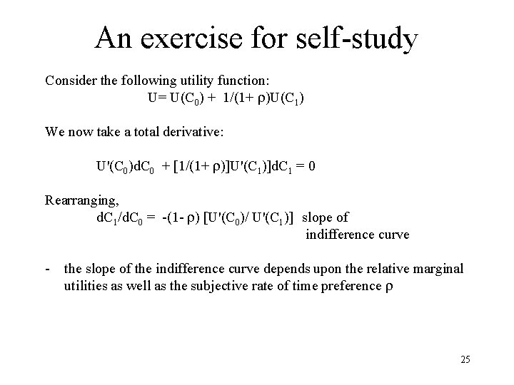
An exercise for self-study Consider the following utility function: U= U(C 0) + 1/(1+ )U(C 1) We now take a total derivative: U'(C 0)d. C 0 + [1/(1+ )]U'(C 1)]d. C 1 = 0 Rearranging, d. C 1/d. C 0 = -(1 - ) [U'(C 0)/ U'(C 1)] slope of indifference curve - the slope of the indifference curve depends upon the relative marginal utilities as well as the subjective rate of time preference 25

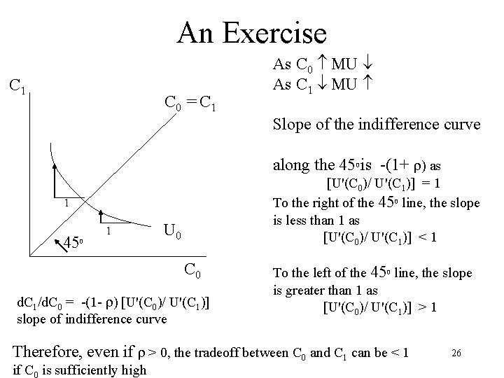
An Exercise C 1 C 0 = C 1 As C 0 MU As C 1 MU Slope of the indifference curve along the 45 is -(1+ ) as 0 [U'(C 0)/ U'(C 1)] = 1 To the right of the 450 line, the slope is less than 1 as [U'(C 0)/ U'(C 1)] < 1 1 45 1 0 U 0 C 0 d. C 1/d. C 0 = -(1 - ) [U'(C 0)/ U'(C 1)] slope of indifference curve To the left of the 450 line, the slope is greater than 1 as [U'(C 0)/ U'(C 1)] > 1 Therefore, even if > 0, the tradeoff between C 0 and C 1 can be < 1 if C 0 is sufficiently high 26

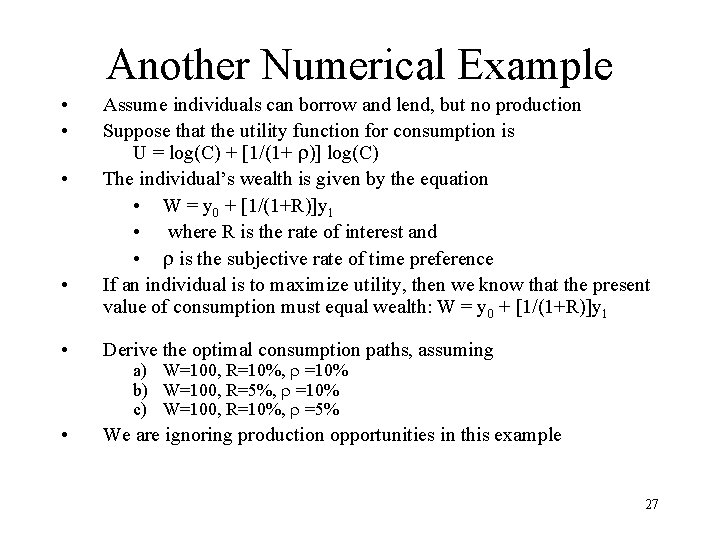
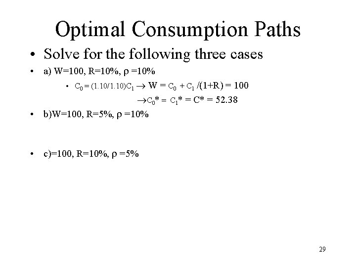
Another Numerical Example • • Assume individuals can borrow and lend, but no production Suppose that the utility function for consumption is U = log(C) + [1/(1+ )] log(C) The individual’s wealth is given by the equation • W = y 0 + [1/(1+R)]y 1 • where R is the rate of interest and • is the subjective rate of time preference If an individual is to maximize utility, then we know that the present value of consumption must equal wealth: W = y 0 + [1/(1+R)]y 1 • Derive the optimal consumption paths, assuming • We are ignoring production opportunities in this example a) W=100, R=10%, =10% b) W=100, R=5%, =10% c) W=100, R=10%, =5% 27

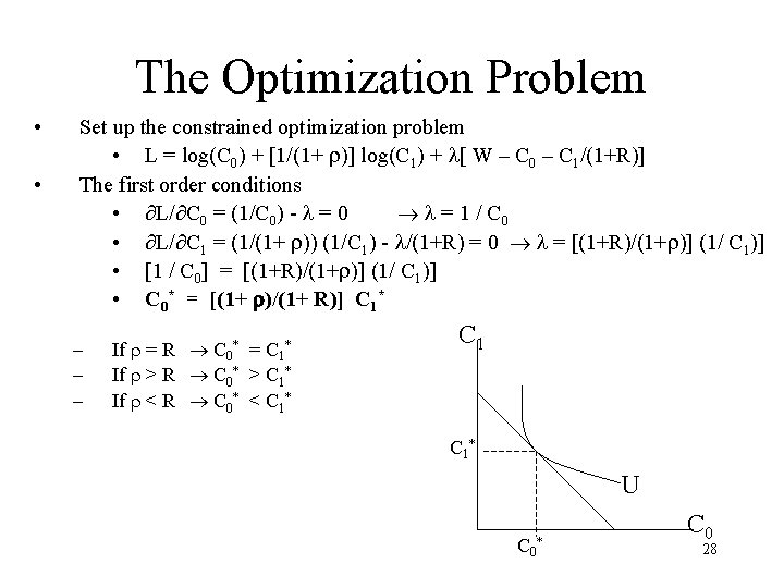
The Optimization Problem • • Set up the constrained optimization problem • L = log(C 0) + [1/(1+ )] log(C 1) + [ W – C 0 – C 1/(1+R)] The first order conditions • L/ C 0 = (1/C 0) - = 0 = 1 / C 0 • L/ C 1 = (1/(1+ )) (1/C 1) - /(1+R) = 0 = [(1+R)/(1+ )] (1/ C 1)] • [1 / C 0] = [(1+R)/(1+ )] (1/ C 1)] • C 0* = [(1+ )/(1+ R)] C 1* – – – If = R C 0* = C 1* If > R C 0* > C 1* If < R C 0* < C 1* C 1 * U C 0 * C 0 28

Optimal Consumption Paths • Solve for the following three cases • a) W=100, R=10%, =10% • C 0 = (1. 10/1. 10)C 1 W = C 0 + C 1 /(1+R) = 100 C 0* = C 1* = C* = 52. 38 • b)W=100, R=5%, =10% • c)=100, R=10%, =5% 29