Interprocedural Analysis Interprocedural Analysis n n Currently we

Interprocedural Analysis

Interprocedural Analysis n n Currently, we only perform data-flow analysis on procedures one at a time. Such analyses are called intraprocedural analyses. An interprocedural analysis operates across an entire program, flowing information from the caller to its callees and vice versa.

Call Graphs n n A call graph for a program is a set of nodes and edges such that There is one node for each procedure in the program. There is one node for each call site, that is, a place in the program where a procedure is invoked. If call site c may call procedure p, then there is an edge from the node for c to the node for p.

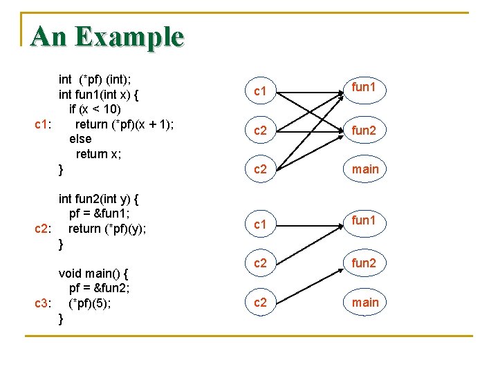
An Example int (*pf) (int); int fun 1(int x) { if (x < 10) c 1: return (*pf)(x + 1); else return x; } int fun 2(int y) { pf = &fun 1; c 2: return (*pf)(y); } void main() { pf = &fun 2; c 3: (*pf)(5); } c 1 fun 1 c 2 fun 2 c 2 main

Context Sensitivity n Interprocedural analysis is challenging because the behavior of each procedure is dependent upon the context in which it is called.

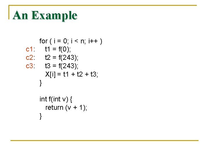
An Example for ( i = 0; i < n; i++ ) c 1: t 1 = f(0); c 2: t 2 = f(243); c 3: t 3 = f(243); X[i] = t 1 + t 2 + t 3; } int f(int v) { return (v + 1); }

Context-Insensitive Analysis n n n We create a super control-flow graph. besides the normal intraprocedural controlflow edges, additional edges are created. Each call site is connected to the beginning of the procedure it calls, and The return statements is connected back to the call sites

A Logical Representation of Data Flow n n n To this point, our representation of data-flow problems and solutions can be termed settheoretic. To cope with the complexity of interprocedural analysis, we now introduce a more general and succinct notation based on logic. Instead of saying something like “definition D is in IN[B], we shall use a notation like in(B, D) to mean the same thing.

A Logical Representation of Data Flow n n n Doing so allows us to express succinct rules about inferring program facts. It also allows us to implement these rules efficiently, in a way that generalizes the bitvector approach to set-theoretic operations. It also allows us to combine what appear to be several independent analyses into one integrated algorithm

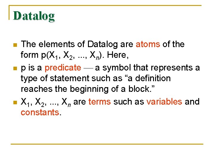
Datalog n n n The elements of Datalog are atoms of the form p(X 1, X 2, . . . , Xn). Here, p is a predicate a symbol that represents a type of statement such as “a definition reaches the beginning of a block. ” X 1, X 2, . . . , Xn are terms such as variables and constants.

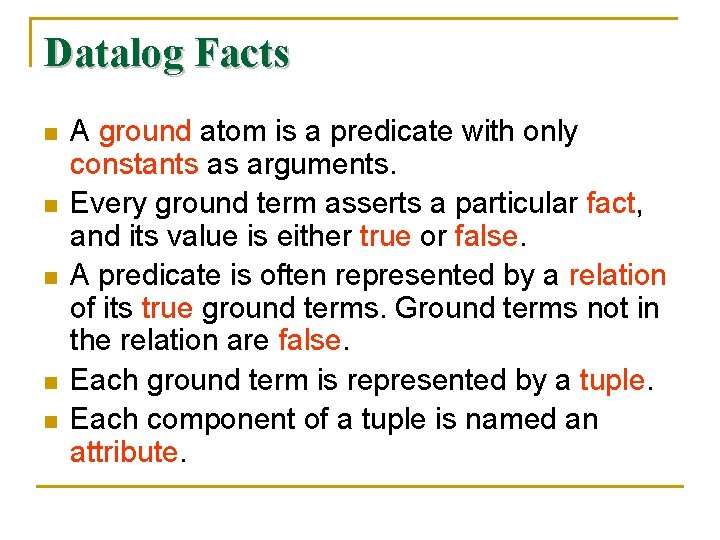
Datalog Facts n n n A ground atom is a predicate with only constants as arguments. Every ground term asserts a particular fact, and its value is either true or false. A predicate is often represented by a relation of its true ground terms. Ground terms not in the relation are false. Each ground term is represented by a tuple. Each component of a tuple is named an attribute.

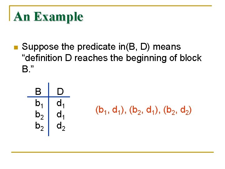
An Example n Suppose the predicate in(B, D) means “definition D reaches the beginning of block B. ” B b 1 b 2 D d 1 d 2 (b 1, d 1), (b 2, d 2)

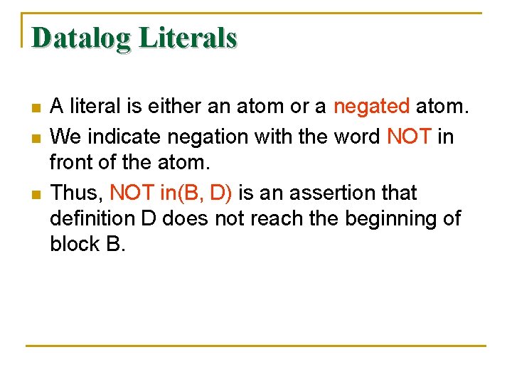
Datalog Literals n n n A literal is either an atom or a negated atom. We indicate negation with the word NOT in front of the atom. Thus, NOT in(B, D) is an assertion that definition D does not reach the beginning of block B.

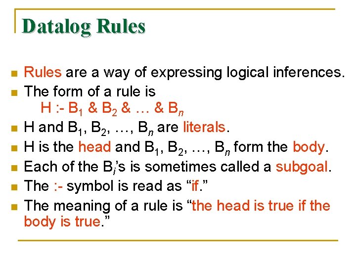
Datalog Rules n n n n Rules are a way of expressing logical inferences. The form of a rule is H : - B 1 & B 2 & … & Bn H and B 1, B 2, …, Bn are literals. H is the head and B 1, B 2, …, Bn form the body. Each of the Bi’s is sometimes called a subgoal. The : - symbol is read as “if. ” The meaning of a rule is “the head is true if the body is true. ”

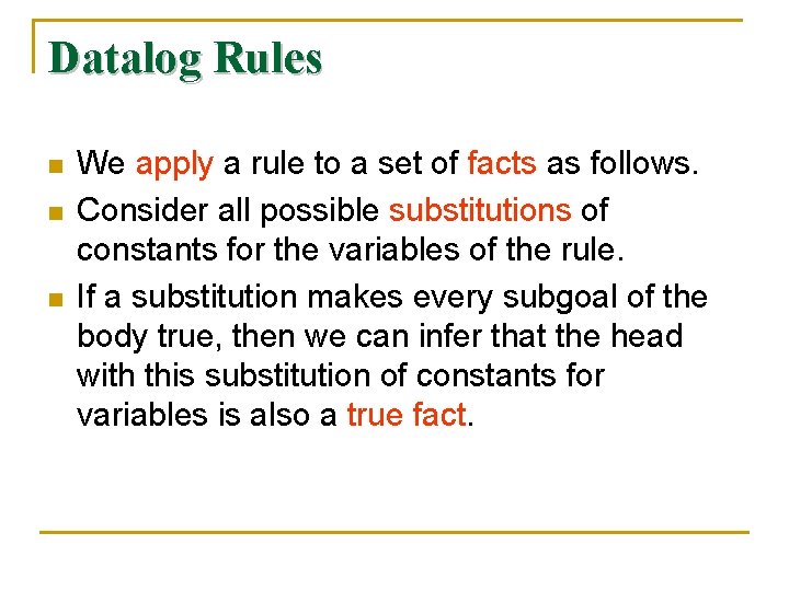
Datalog Rules n n n We apply a rule to a set of facts as follows. Consider all possible substitutions of constants for the variables of the rule. If a substitution makes every subgoal of the body true, then we can infer that the head with this substitution of constants for variables is also a true fact.

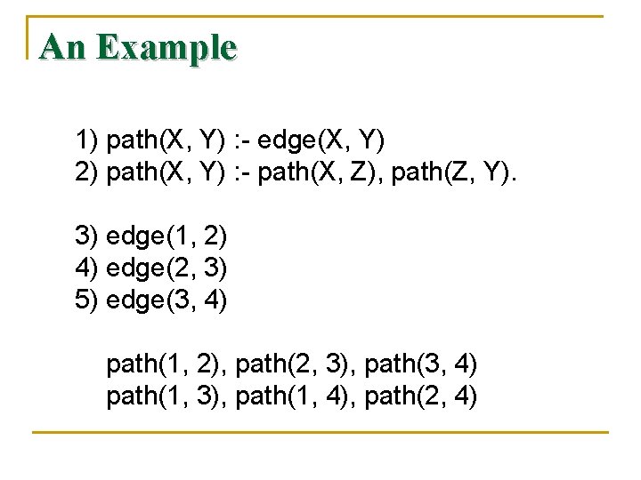
An Example 1) path(X, Y) : - edge(X, Y) 2) path(X, Y) : - path(X, Z), path(Z, Y). 3) edge(1, 2) 4) edge(2, 3) 5) edge(3, 4) path(1, 2), path(2, 3), path(3, 4) path(1, 3), path(1, 4), path(2, 4)

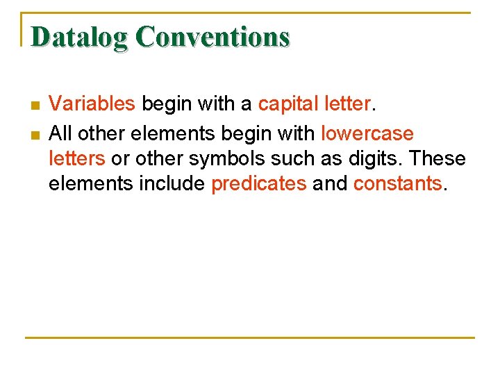
Datalog Conventions n n Variables begin with a capital letter. All other elements begin with lowercase letters or other symbols such as digits. These elements include predicates and constants.

Why is Pointer Analysis Difficult n n Pointer analysis in C is particularly difficult, because C programs can perform arbitrary computations on pointers. Pointers in Java are much simpler. Pointer analysis must be interprocedural. Languages allowing indirect function calls present an additional challenge. Virtual methods in Java cause many invocations to be indirect.

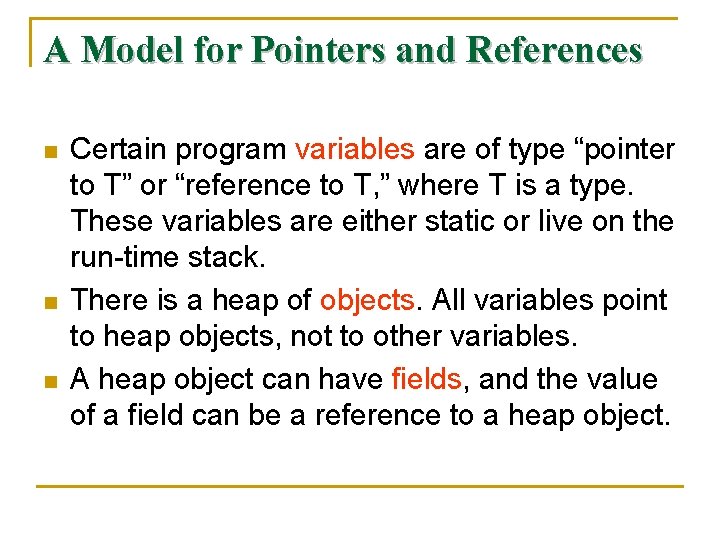
A Model for Pointers and References n n n Certain program variables are of type “pointer to T” or “reference to T, ” where T is a type. These variables are either static or live on the run-time stack. There is a heap of objects. All variables point to heap objects, not to other variables. A heap object can have fields, and the value of a field can be a reference to a heap object.

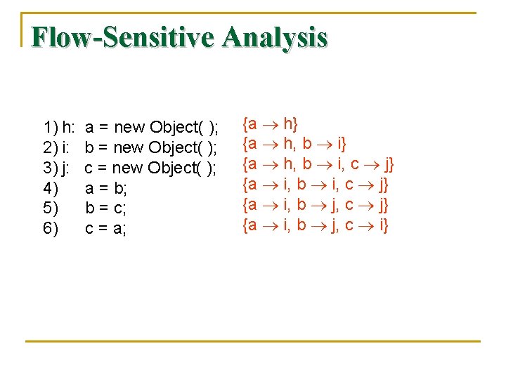
Flow-Sensitive Analysis 1) h: 2) i: 3) j: 4) 5) 6) a = new Object( ); b = new Object( ); c = new Object( ); a = b; b = c; c = a; {a h} {a h, b i, c j} {a i, b j, c i}

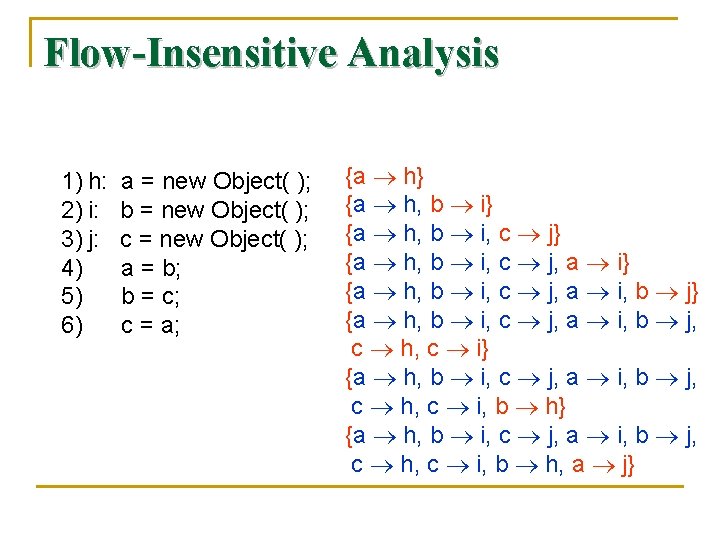
Flow-Insensitive Analysis 1) h: 2) i: 3) j: 4) 5) 6) a = new Object( ); b = new Object( ); c = new Object( ); a = b; b = c; c = a; {a h} {a h, b i, c j} {a h, b i, c j, a i, b j, c h, c i, b h} {a h, b i, c j, a i, b j, c h, c i, b h, a j}

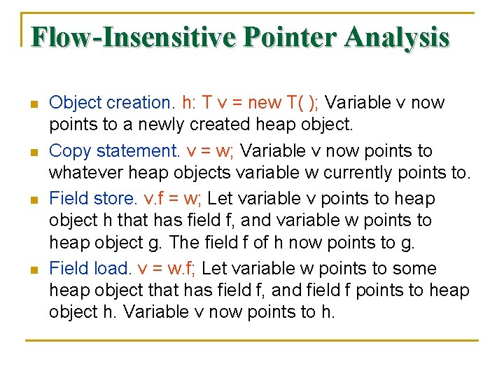
Flow-Insensitive Pointer Analysis n n Object creation. h: T v = new T( ); Variable v now points to a newly created heap object. Copy statement. v = w; Variable v now points to whatever heap objects variable w currently points to. Field store. v. f = w; Let variable v points to heap object h that has field f, and variable w points to heap object g. The field f of h now points to g. Field load. v = w. f; Let variable w points to some heap object that has field f, and field f points to heap object h. Variable v now points to h.

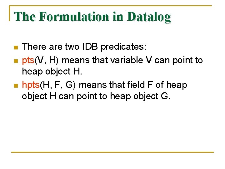
The Formulation in Datalog n n n There are two IDB predicates: pts(V, H) means that variable V can point to heap object H. hpts(H, F, G) means that field F of heap object H can point to heap object G.

The Formulation in Datalog n n pts(V, H) : - “H: T V = new T()” pts(V, H) : - “V = W” & pts(W, H) hpts(H, F, G) : - “V. F = W” & pts(W, G) & pts(V, H) : - “V = W. F” & pts(W, G) & hpts(G, F, H) Simplified EDB facts

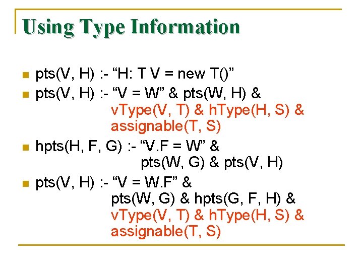
Using Type Information n n Because Java is type safe, variables can only point to types that are compatible to the declared types. We introduce the following three EDB predicates: v. Type(V, T) says that variable V is declared to have type T. h. Type(H, T) says that heap object H is allocated with type T. assignable(T, S) means that an object of type S can be assigned to a variable with the type T. assignable(T, T) is always true.

Using Type Information n n pts(V, H) : - “H: T V = new T()” pts(V, H) : - “V = W” & pts(W, H) & v. Type(V, T) & h. Type(H, S) & assignable(T, S) hpts(H, F, G) : - “V. F = W” & pts(W, G) & pts(V, H) : - “V = W. F” & pts(W, G) & hpts(G, F, H) & v. Type(V, T) & h. Type(H, S) & assignable(T, S)

Context-Insensitive Interprocedural Pointer Analysis n n n We now consider method invocations. We first explain how points-to analysis can be used to compute a precise call graph, which is useful in computing precise points-to results. We then formalize on-the-fly call-graph discovery and show Datalog can be used to describe the analysis succinctly.

Effects of a Method Invocation n n The effects of a method call, x = y. n(z), can be computed in 3 steps: First, determine the type of the receiver object, which is the object that y points to. Suppose its type is t. let m be the method named n in the narrowest superclass of t that has a method named n.

Effects of a Method Invocation n Second, the formal parameters of m are assigned the objects pointed to by the actual parameters. The actual parameters include not just the parameters passed indirectly, but also the receiver object itself. Every method invocation assigns the receiver object to the this variable. We refer to the this variables as the 0 th formal parameters of methods.

Effects of a Method Invocation n Third, the returned object of m is assigned to the left-hand-side variable of the assignment statement.

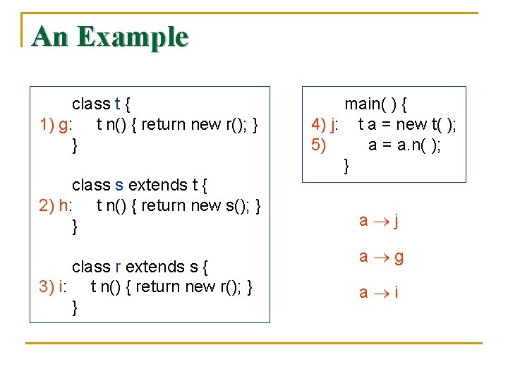
An Example class t { 1) g: t n() { return new r(); } } class s extends t { 2) h: t n() { return new s(); } } class r extends s { 3) i: t n() { return new r(); } } main( ) { 4) j: t a = new t( ); 5) a = a. n( ); } a j a g a i

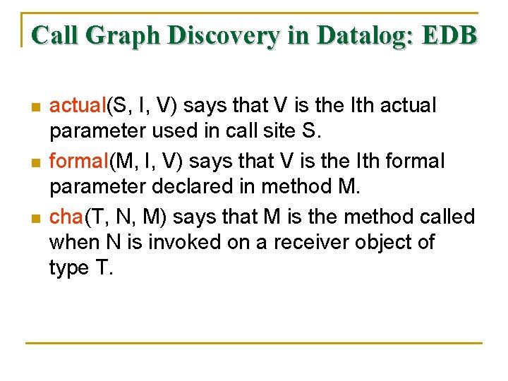
Call Graph Discovery in Datalog: EDB n n n actual(S, I, V) says that V is the Ith actual parameter used in call site S. formal(M, I, V) says that V is the Ith formal parameter declared in method M. cha(T, N, M) says that M is the method called when N is invoked on a receiver object of type T.

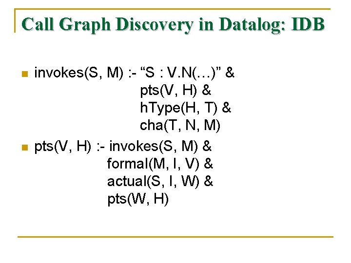
Call Graph Discovery in Datalog: IDB n n invokes(S, M) : - “S : V. N(…)” & pts(V, H) & h. Type(H, T) & cha(T, N, M) pts(V, H) : - invokes(S, M) & formal(M, I, V) & actual(S, I, W) & pts(W, H)

Context-Sensitive Interprocedural Pointer Analysis n n n We will discuss a cloning-based contextsensitive analysis. A cloning-based analysis simply clones the methods, one for each context of interest. We then apply the context-insensitive analysis to the cloned call graph.

Contexts and Call Strings n n n A context is a representation of the call strings that forms the history of the active function calls. A context is a summary of the sequence of calls whose activation records are currently on the run-time stack. If there are no recursive functions on the stack, then the call string is a complete representation.

Contexts and Call Strings n n If there are recursive functions in the program, then the number of possible call string is infinite. Here, we shall adopt a simple scheme that captures the history of nonrecursive calls but considers recursive calls to be “too hard to unravel. ”

Contexts and Call Strings n n n Consider a graph whose nodes are the functions, with an edge from p to q if p calls q. The strongly connected components (SCC’s) of this graph are the sets of mutually recursive functions. Call an SCC nontrivial if it either has more than one member, or it has a single recursive member.

Contexts and Call Strings n n Given a call string, delete the occurrence of a call site s if s is in a function p. Function q is called at site s (q = p is possible). p and q are in the same strongly connected component (i. e. , p and q are mutually recursive, or p = q and p is recursive).

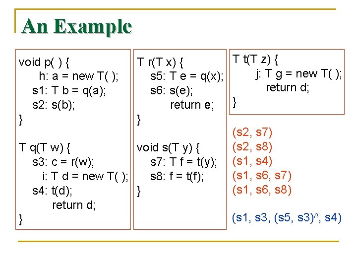
An Example T t(T z) { T r(T x) { j: T g = new T( ); s 5: T e = q(x); return d; s 6: s(e); } return e; } (s 2, s 7) (s 2, s 8) T q(T w) { void s(T y) { s 3: c = r(w); s 7: T f = t(y); (s 1, s 4) (s 1, s 6, s 7) i: T d = new T( ); s 8: f = t(f); (s 1, s 6, s 8) s 4: t(d); } return d; (s 1, s 3, (s 5, s 3)n, s 4) } void p( ) { h: a = new T( ); s 1: T b = q(a); s 2: s(b); }

Cloned Call Graph n n We now describe how we derive the cloned call graph. Each cloned method is identified by the method in the program M and a context C. Edges can be derived by adding the corresponding contexts to each of the edges in the original call graph Define a CSinvokes predicate such that CSinvokes(S, C, M, D) is true if the call site S in context C calls the D context of method M.

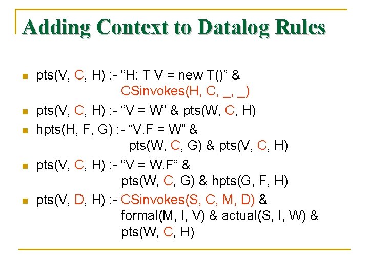
Adding Context to Datalog Rules n n n pts(V, C, H) : - “H: T V = new T()” & CSinvokes(H, C, _, _) pts(V, C, H) : - “V = W” & pts(W, C, H) hpts(H, F, G) : - “V. F = W” & pts(W, C, G) & pts(V, C, H) : - “V = W. F” & pts(W, C, G) & hpts(G, F, H) pts(V, D, H) : - CSinvokes(S, C, M, D) & formal(M, I, V) & actual(S, I, W) & pts(W, C, H)

Binary Decision Diagrams n n n Binary Decision Diagrams (BDD’s) are a method for representing boolean functions by graphs. n 2 Since there are 2 boolean functions of n variables, no representation method is going to be very succinct on all boolean functions. However, the boolean functions that appear in practice tend to have a lot of regularity. It is thus common that one can find a succinct BDD for functions that one really wants to represent.

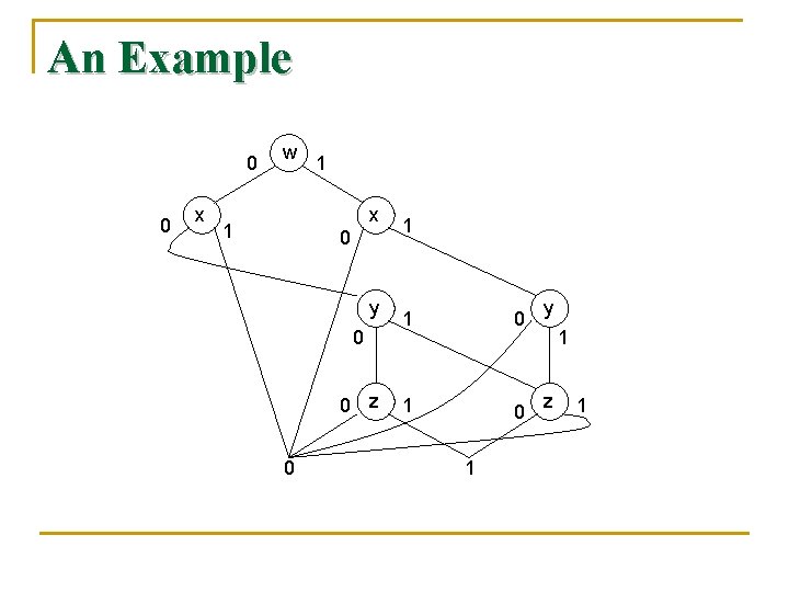
Binary Decision Diagrams n n n A BDD represents a boolean function by a rooted DAG. The interior nodes of the DAG are each labeled by one of the variables of the represented function. At the bottom are two leaves, one labeled 0 and the other labeled 1. Each interior node has two edges to children; these edges are called “low” and “high. ” The low edge corresponds to the case where the variable has value 0, and the high edge value 1.

Binary Decision Diagrams n n Given a truth assignment for the variables, we can start at the root, say a node labeled x, follow the low or high edge, depending on whether the truth value for x is 0 or 1, respectively. If we arrive at the leaf labeled 1, then the represented function is true for this truth assignment; otherwise it is false.

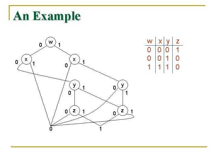
An Example 0 0 x w x 1 0 y 0 0 z 0 w 0 0 1 1 0 1 y 1 z 1 x 0 0 1 y 0 1 1 z 1 0 0

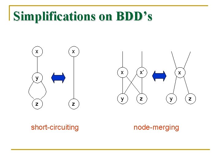
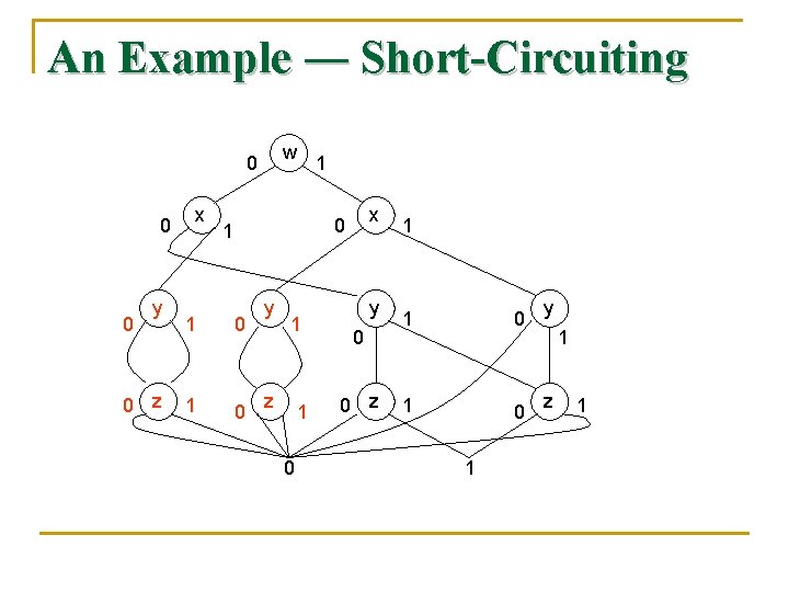
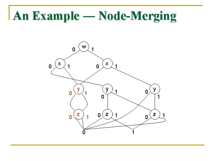
Simplifications on BDD’s n n Short-Circuiting: If a node N has both its high and low edges go to the same node M, then we may eliminate N. Edges entering N go to M instead. Node-Merging: If two nodes N and M have low edges that go to the same node and also have high edges that go to the same node, then we may merge N with M. Edges entering either N or M go to the merged node.

Simplifications on BDD’s x x y z z short-circuiting x x’ y z x y node-merging z

An Example 0 0 x w 1 x 1 0 y 0 0 z 0 1 1 0 1 y 1 z 1

An Example ― Short-Circuiting w 0 0 0 y 0 z x 1 x 0 1 1 0 y 1 z 1 0 y 0 0 z 1 1 0 1 y 1 z 1

An Example ― Node-Merging w 0 0 x 1 1 0 0 x 0 y 1 z 1 0 y 0 0 z 1 1 0 1 y 1 z 1

Representing Relations by BDD’s n n n The relations with which we have been dealing have components that are taken from “domains. ” A domain for a component of a relation is the set of possible values that tuples can have in that component. If a domain has more than 2 n-1 possible values but no more than 2 n values, then it requires n bits or boolean variables to represent values in that domain.

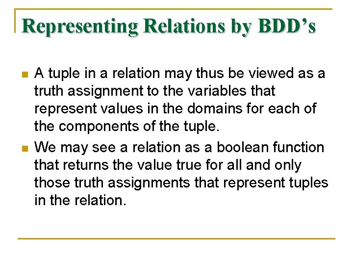
Representing Relations by BDD’s n n A tuple in a relation may thus be viewed as a truth assignment to the variables that represent values in the domains for each of the components of the tuple. We may see a relation as a boolean function that returns the value true for all and only those truth assignments that represent tuples in the relation.

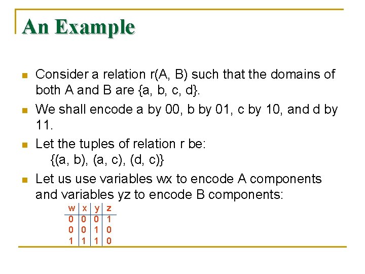
An Example n n Consider a relation r(A, B) such that the domains of both A and B are {a, b, c, d}. We shall encode a by 00, b by 01, c by 10, and d by 11. Let the tuples of relation r be: {(a, b), (a, c), (d, c)} Let us use variables wx to encode A components and variables yz to encode B components: w 0 0 1 x 0 0 1 y 0 1 1 z 1 0 0

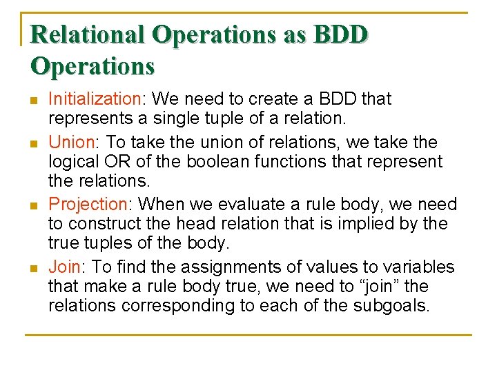
Relational Operations as BDD Operations n n Initialization: We need to create a BDD that represents a single tuple of a relation. Union: To take the union of relations, we take the logical OR of the boolean functions that represent the relations. Projection: When we evaluate a rule body, we need to construct the head relation that is implied by the true tuples of the body. Join: To find the assignments of values to variables that make a rule body true, we need to “join” the relations corresponding to each of the subgoals.