Interpolation Tools Lesson 5 overview q Concepts Sampling

Interpolation Tools

Lesson 5 overview q Concepts § § Sampling methods Creating continuous surfaces Interpolation Density surfaces in GIS q Interpolators § IDW, Spline, Trend, Kriging, Natural neighbors § Topo. To. Raster q Assessing accuracy q Exercise 5

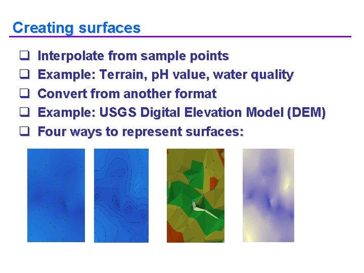
Creating surfaces q q q Interpolate from sample points Example: Terrain, p. H value, water quality Convert from another format Example: USGS Digital Elevation Model (DEM) Four ways to represent surfaces:

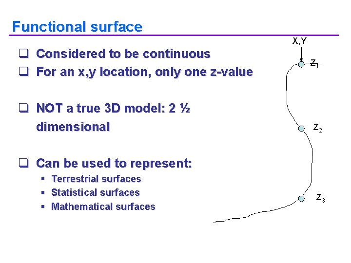
Functional surface X, Y q Considered to be continuous q For an x, y location, only one z-value q NOT a true 3 D model: 2 ½ dimensional Z 1 Z 2 q Can be used to represent: § § § Terrestrial surfaces Statistical surfaces Mathematical surfaces Z 3

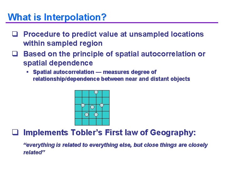
What is Interpolation? q Procedure to predict value at unsampled locations within sampled region q Based on the principle of spatial autocorrelation or spatial dependence § Spatial autocorrelation — measures degree of relationship/dependence between near and distant objects q Implements Tobler’s First law of Geography: “everything is related to everything else, but close things are closely related”

Elements of interpolation q The known points (samples) § Sample factors - size, Iimits, location , outliers q The unknown points (interpolated values) § Interpolation models: • Deterministic - create surfaces from measured points, based on either the extent of similarity (IDW) or degree of smoothing (Trend). • Geostatistical - based on statistics (Kriging) with advanced prediction modeling, includes measure of certainty or accuracy of predictions. q Different interpolation methods will (almost always) produce different results.

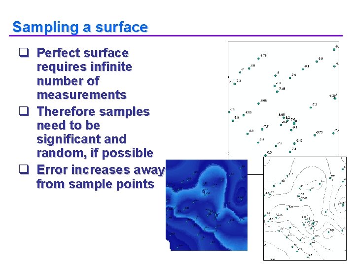
Sampling a surface q Perfect surface requires infinite number of measurements q Therefore samples need to be significant and random, if possible q Error increases away from sample points

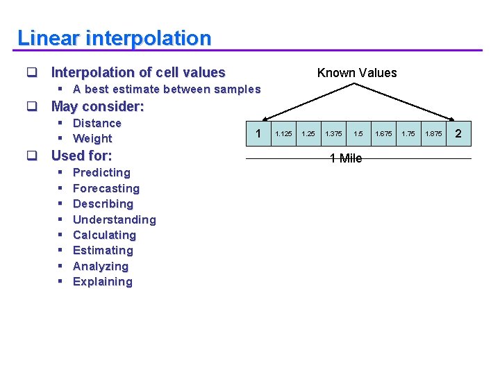
Linear interpolation q Interpolation of cell values Known Values § A best estimate between samples q May consider: § Distance § Weight q Used for: § § § § Predicting Forecasting Describing Understanding Calculating Estimating Analyzing Explaining 1 1. 125 1. 375 1. 5 1 Mile 1. 675 1. 875 2

Controlling sample points for interpolation q IDW, Spline & Kriging support control of sample numbers q Sample methods: § Nearest neighbors — you choose how many § Search radius — variable or max distance q Returns No. Data if insufficient samples

Barriers to interpolation q Barriers represented by line feature classes § Examples: Faults, cliffs, levees, depth to ground water q Restricts samples to same side of line as cell q IDW, KRIGING ()support barriers

Interpolating unknown values q Input § Point dataset § x, y coordinates in a text file q Output § Floating-point raster q Tools

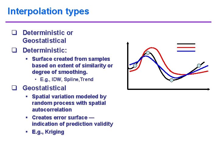
Interpolation types q Deterministic or Geostatistical q Deterministic: § Surface created from samples based on extent of similarity or degree of smoothing. • E. g. , IDW, Spline, Trend q Geostatistical § Spatial variation modeled by random process with spatial autocorrelation § Creates error surface — indication of prediction validity § E. g. , Kriging

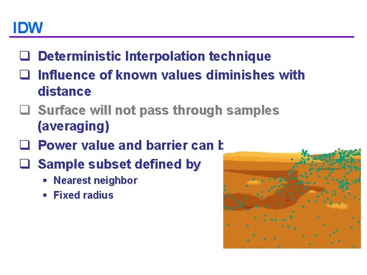
IDW q Deterministic Interpolation technique q Influence of known values diminishes with distance q Surface will not pass through samples (averaging) q Power value and barrier can be used q Sample subset defined by § Nearest neighbor § Fixed radius

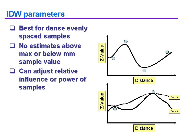
Distance Z-Value q Best for dense evenly spaced samples q No estimates above max or below mm sample value q Can adjust relative influence or power of samples Z-Value l. DW parameters Power 1 Power 2 Distance

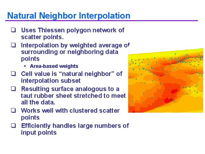
Natural Neighbor Interpolation q Uses Thiessen polygon network of scatter points. q Interpolation by weighted average of surrounding or neighboring data points § Area-based weights q Cell value is “natural neighbor” of interpolation subset q Resulting surface analogous to a taut rubber sheet stretched to meet all the data. q Works well with clustered scatter points q Efficiently handles large numbers of input points

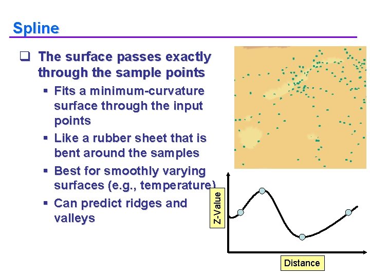
Spline q The surface passes exactly through the sample points Z-Value § Fits a minimum-curvature surface through the input points § Like a rubber sheet that is bent around the samples § Best for smoothly varying surfaces (e. g. , temperature) § Can predict ridges and valleys Distance

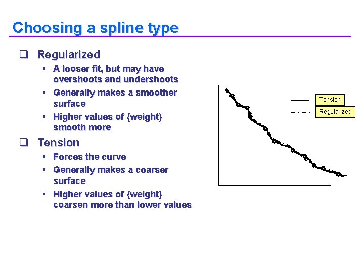
Choosing a spline type q Regularized § A looser fit, but may have overshoots and undershoots § Generally makes a smoother surface § Higher values of {weight} smooth more q Tension § Forces the curve § Generally makes a coarser surface § Higher values of {weight} coarsen more than lower values Tension Regularized

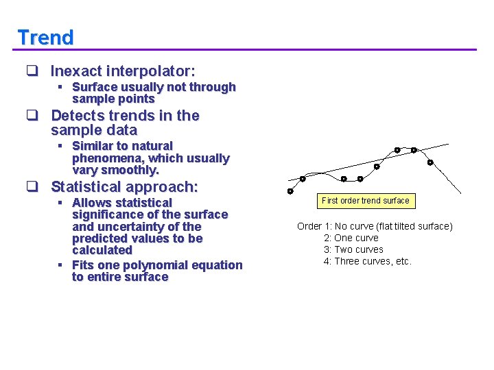
Trend q Inexact interpolator: § Surface usually not through sample points q Detects trends in the sample data § Similar to natural phenomena, which usually vary smoothly. q Statistical approach: § Allows statistical significance of the surface and uncertainty of the predicted values to be calculated § Fits one polynomial equation to entire surface First order trend surface Order 1: No curve (flat tilted surface) 2: One curve 3: Two curves 4: Three curves, etc.

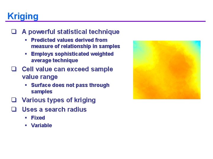
Kriging q A powerful statistical technique § Predicted values derived from measure of relationship in samples § Employs sophisticated weighted average technique q Cell value can exceed sample value range § Surface does not pass through samples q Various types of kriging q Uses a search radius § Fixed § Variable

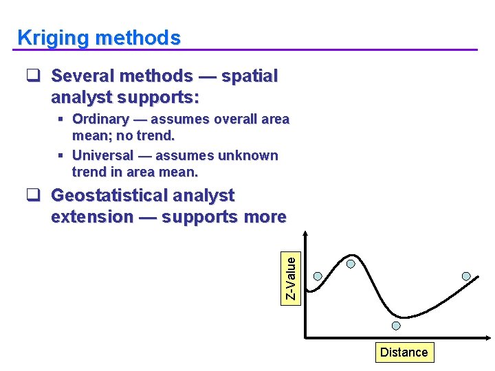
Kriging methods q Several methods — spatial analyst supports: § Ordinary — assumes overall area mean; no trend. § Universal — assumes unknown trend in area mean. Z-Value q Geostatistical analyst extension — supports more Distance

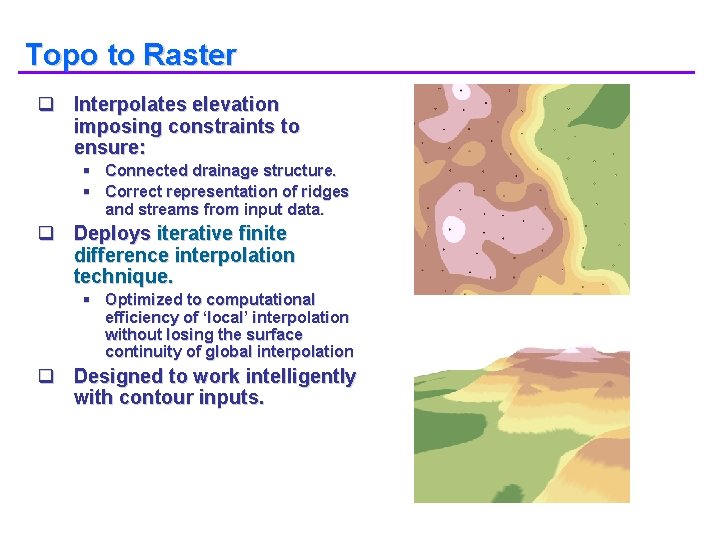
Topo to Raster q Interpolates elevation imposing constraints to ensure: § Connected drainage structure. § Correct representation of ridges and streams from input data. q Deploys iterative finite difference interpolation technique. § Optimized to computational efficiency of ‘local’ interpolation without losing the surface continuity of global interpolation q Designed to work intelligently with contour inputs.

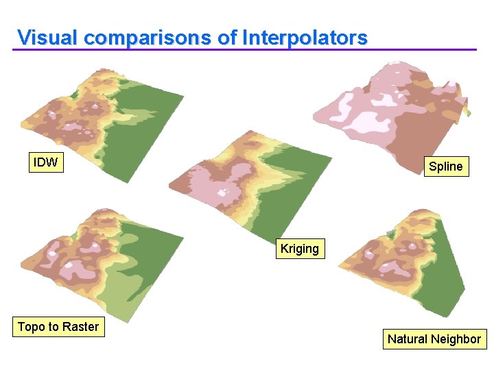
Visual comparisons of Interpolators IDW Spline Kriging Topo to Raster Natural Neighbor

Feature density estimation q Count occurrences of a phenomena within an area and distribute it through the area § Similar to focal functions § Performs statistics on features § Population field influences density q Use points or lines as input q Examples § § § Population per square kilometer Road density per square mile The number of customers per square mile

Testing your surface q Different interpolators will produce different results with same input data. q No single method is more accurate than others for all situations. q Accuracy — may be determined by comparison with a second set of “withheld” samples for accuracy checking. § § § q Remove random test sample points Create surface Interpolate Did interpolator predict missing samples? Repeat Try with each interpolator Select the method based on knowledge of the study area, phenomena of interest, and available resources.